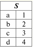
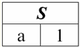
Lecture No. 5. Relational algebra. Binary Operations

1. Operations of union, intersection, difference

Any operations have their own applicability rules that must be observed so that expressions and actions do not lose their meaning. The binary set-theoretic operations of union, intersection, and difference can only be applied to two relations necessarily with the same relation schema. The result of such binary operations will be relations consisting of tuples that satisfy the conditions of the operations, but with the same relation scheme as the operands.

1. The result union operations two relations r₁(S) and r₂(S) there will be a new relation r₃(S) consisting of those tuples of relations r₁(S) and r₂(S) that belong to at least one of the original relations and with the same relationship schema.

So the intersection of the two relations is:

r₃(S) = r₁(S) r₂(S) = {t(S) | t ∈r₁ ∪t ∈r₂};

For clarity, here is an example in terms of tables:

Let two relations be given:

r₁(S):

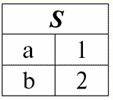
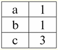
r₂(S):

We see that the schemes of the first and second relations are the same, only they have a different number of tuples. The union of these two relations will be the relation r₃(S), which will correspond to the following table:

r3(S) = r₁(S) r₂(S):

So, the schema of relation S has not changed, only the number of tuples has increased.

2. Let's move on to the consideration of the next binary operation - intersection operations two relationships. As we know from school geometry, the resulting relation will include only those tuples of the original relations that are present simultaneously in both relations r₁(S) and r₂(S) (again, note the same relationship pattern).

The operation of the intersection of two relations will look like this:

r₄(S) = r₁(S)∩r₂(S) = {t(S) | t ∈ r₁ & t ∈ r₂};

And again, consider the effect of this operation on relations presented in the form of tables:

r₁(S):

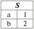
r₂(S):

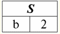
According to the definition of the operation by the intersection of relations r₁(S) and r₂(S) there will be a new relation r₄(S), whose table view would look like this:

r₄(S) = r₁(S)∩r₂(S):

Indeed, if we look at the tuples of the first and second initial relations, there is only one common among them: {b, 2}. It became the only tuple of the new relation r₄(S).

3. Difference operation two relations is defined in a similar way to the previous operations. Operand relations, as in the previous operations, must have the same relation schemes, then the resulting relation will include all those tuples of the first relation that are not in the second, i.e.:

r₅(S) = r₁(S)\r₂(S) = {t(S) | t ∈ r₁ & t ∉ r₂};

The already well-known relations r₁(S) and r₂(S), in a tabular view looking like this:

r₁(S):

r₂(S):

We will consider both operands in the operation of the intersection of two relations. Then, following this definition, the resulting relation r5(S) will look like this:

r₅(S) = r₁(S)\r₂(S):

The considered binary operations are basic, other operations, more complex, are based on them.

2. Cartesian product and natural join operations

The Cartesian product operation and the natural join operation are binary operations of the product type and are based on the union of two relations operation that we discussed earlier.

Although the action of the Cartesian product operation may seem familiar to many, we will nevertheless begin with the natural product operation, since it is a more general case than the first operation.

So, consider the natural join operation. It should be immediately noted that the operands of this action can be relations with different schemes, in contrast to the three binary operations of union, intersection and renaming.

If we consider two relations with different relation schemes r₁(S₁) and r₂(S₂), then their natural compound there will be a new relation r₃(S₃), which will consist only of those tuples of operands that match at the intersection of relationship schemes. Accordingly, the scheme of the new relationship will be larger than any of the schemes of relations of the original ones, since it is their connection, "gluing". By the way, tuples that are identical in two operand relations, according to which this "gluing" occurs, are called connectable.

Let's write the definition of the natural join operation in the formula language of database management systems:

r₃(S₃) = r₁(S₁)xr₂(S₂) = {t(S₁ ∪S₂) | t[S₁] ∈ r₁ &t(S₂) ∈ r₂};

Let's consider an example that well illustrates the work of a natural connection, its "gluing". Let two relations r₁(S₁) and r₂(S₂), in the tabular form of representation, respectively, equal:

r₁(S₁):

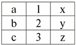
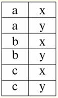
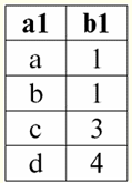
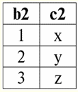
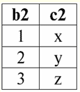
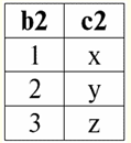
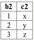
r₂(S₂):

We see that these relations have tuples that coincide at the intersection of schemes S₁ and S₂ relations. Let's list them:

1) tuple {a, 1} of relation r₁(S₁) matches the tuple {1, x} of the relation r₂(S₂);

2) tuple {b, 1} from r₁(S₁) also matches the tuple {1, x} from r₂(S₂);

3) the tuple {c, 3} matches the tuple {3, z}.

Hence, under natural join, the new relation r₃(S₃) is obtained by "gluing" exactly on these tuples. So r₃(S₃) in a table view will look like this:

r₃(S₃) = r₁(S₁)xr₂(S₂):

It turns out by definition: scheme S₃ does not coincide with the scheme S₁, nor with the scheme S₂, we "glued" the two original schemas by intersecting tuples to get their natural join.

Let us show schematically how tuples are joined when applying the natural join operation.

Let the relation r₁ has a conditional form:

And the ratio r₂ - view:

Then their natural connection would look like this:

We see that the "gluing" of relations-operands occurs according to the same scheme that we gave earlier, considering the example.

Operation Cartesian connection is a special case of the natural join operation. More specifically, when considering the effect of the operation of the Cartesian product on relations, we deliberately stipulate that in this case we can only talk about non-intersecting relation schemes. As a result of applying both operations, relations with schemas equal to the union of schemas of operand relations are obtained, only all possible pairs of their tuples fall into the Cartesian product of two relations, since the schemas of operands should in no case intersect.

Thus, based on the foregoing, we write a mathematical formula for the Cartesian product operation:

r₄(S₄) = r₁(S1)xr₂(S₂) = {t(S₁ ∪S₂) | t[S₁] ∈ r₁ &t(S₂) ∈ r₂}, S₁ S₂= ∅;

Now let's look at an example to show how the resulting relation schema will look when applying the Cartesian product operation.

Let two relations r₁(S1) and r₂(S₂), which are presented in tabular form as follows:

r₁(S₁):

r₂(S₂):

So we see that none of the tuples of relations r₁(S₁) and r₂(S₂), indeed, does not coincide in their intersection. Therefore, in the resulting relation r₄(S₄) all possible pairs of tuples of the first and second operand relations will fall. Get:

r₄(S₄) = r₁(S1)xr₂(S₂):

We have obtained a new relation scheme r₄(S₄) not by "gluing" tuples as in the previous case, but by enumeration of all possible different pairs of tuples that do not match in the intersection of the original schemes.

Again, as in the case of natural join, we give a schematic example of the operation of the Cartesian product operation.

Let r₁ set as follows:

And the ratio r₂ given:

Then their Cartesian product can be schematically represented as follows:

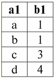
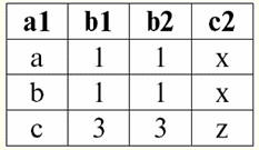
It is in this way that the resulting relation is obtained when applying the operation of the Cartesian product.

3. Properties of binary operations

From the above definitions of the binary operations of union, intersection, difference, Cartesian product, and natural join, properties follow.

1. The first property, as in the case of unary operations, illustrates power ratio relations:

1) for the union operation:

|r₁ ∪r₂| ≤ |r₁| + |r₂|;

2) for the intersection operation:

|r₁ ∩r₂ | ≤ min(|r₁|, |r₂|);

3) for the difference operation:

|r₁ \r₂| ≤ |r₁|;

4) for the Cartesian product operation:

|r₁ xr₂| = |r₁| |r₂|;

5) for natural join operation:

|r₁ xr₂| ≤ |r₁| |r₂|.

The ratio of powers, as we remember, characterizes how the number of tuples in relations changes after applying one or another operation. So what do we see? Power association two relations r₁ and r₂ less than the sum of the cardinalities of the original operand relations. Why is this happening? The thing is that when you merge, matching tuples disappear, overlapping each other. So, referring to the example that we considered after going through this operation, you can see that in the first relation there were two tuples, in the second - three, and in the resulting - four, i.e. less than five (the sum of the cardinalities of the relations-operands ). By the matching tuple {b, 2}, these relations are "glued together".

Result Power intersections two relations is less than or equal to the minimum cardinality of the original operand relations. Let us turn to the definition of this operation: only those tuples that are present in both initial relations get into the resulting relation. This means that the cardinality of the new relation cannot exceed the cardinality of the relation-operand whose number of tuples is the smallest of the two. And the power of the result can be equal to this minimum cardinality, since the case is always allowed when all tuples of a relation with a lower cardinality coincide with some tuples of the second relation-operand.

In case of operation differences everything is quite trivial. Indeed, if all tuples that are also present in the second relation are "subtracted" from the first relation-operand, then their number (and, consequently, their power) will decrease. In the event that not a single tuple of the first relation matches any tuple of the second relation, i.e., there is nothing to "subtract", its power will not decrease.

Interestingly, if the operation Cartesian product the power of the resulting relation is exactly equal to the product of the powers of the two operand relations. It is clear that this happens because all possible pairs of tuples of the original relations are written into the result, and nothing is excluded.

And finally, the operation natural connection a relation is obtained whose cardinality is greater than or equal to the product of the cardinalities of the two original relations. Again, this happens because the operand relations are "glued" by matching tuples, and non-matching ones are excluded from the result altogether.

2. Idempotency property:

1) for the union operation: r ∪ r = r;

2) for the intersection operation: r ∩ r = r;

3) for the difference operation: r \ r ≠ r;

4) for the Cartesian product operation (in the general case, the property is not applicable);

5) for the natural join operation: r x r = r.

Interestingly, the property of idempotency is not true for all of the above operations, and for the operation of the Cartesian product, it is not applicable at all. Indeed, if you combine, intersect, or naturally connect any relation with itself, it will not change. But if you subtract from a relation exactly equal to it, the result will be an empty relation.

3. Commutative property:

1) for the union operation:

r₁ ∪r₂ =r₂ ∪r₁;

2) for the intersection operation:

r ∩ r = r ∩ r;

3) for the difference operation:

r₁ \r₂ ≠r₂ \r₁;

4) for the Cartesian product operation:

r₁ xr₂ =r₂ xr₁;

5) for natural join operation:

r₁ xr₂ =r₂ xr₁.

The commutativity property holds for all operations except for the difference operation. This is easy to understand, because their composition (tuples) does not change from rearranging relations in places. And when applying the difference operation, it is important which of the operand relations comes first, because it depends on which tuples of which relation will be taken as reference, i.e., with which tuples other tuples will be compared for exclusion.

4. Associativity property:

1) for the union operation:

(r₁ ∪r₂)∪r₃ =r₁ ∪(r₂ ∪r₃);

2) for the intersection operation:

(r₁ ∩r₂)∩r₃ =r₁ ∩(r₂ ∩r₃);

3) for the difference operation:

(r₁ \r₂)\r₃ ≠r₁ \(r₂ \r₃);

4) for the Cartesian product operation:

(r₁ xr₂)xr₃ =r₁ x(r₂ xr₃);

5) for natural join operation:

(r₁ xr₂)xr₃ =r₁ x(r₂ xr₃).

And again we see that the property is executed for all operations except for the difference operation. This is explained in the same way as in the case of applying the commutativity property. By and large, the operations of union, intersection, difference, and natural join do not care what order the operand relations are in. But when relationships are "taken away" from each other, order plays a dominant role.

Based on the above properties and reasoning, the following conclusion can be drawn: the last three properties, namely the property of idempotency, commutativity and associativity, are true for all the operations we have considered, except for the operation of the difference of two relations, for which none of the three properties indicated were satisfied at all, and only in one case the property was found to be inapplicable.

4. Connection operation options

Using as a basis the unary operations of selection, projection, renaming and binary operations of union, intersection, difference, Cartesian product and natural join considered earlier (all of them are generally called connection operations), we can introduce new operations derived using the above concepts and definitions. This activity is called compiling. join operation options.

The first such variant of join operations is the operation inner connection according to the specified connection condition.

The operation of an inner join, by some specific condition, is defined as a derivative operation from the operations of the Cartesian product and selection.

We write the formula definition of this operation:

r₁(S₁)x _P r₂(S₂) = σ (r₁ xr₂), St₁ S₂ = ∅;

Here P = P<S₁ ∪S₂> - a condition imposed on the union of two schemes of the original relations-operands. It is by this condition that tuples are selected from the relations r₁ and r₂ into the resulting relation.

Note that the inner join operation can be applied to relationships with different relationship schemas. These schemes can be any, but in no case should they intersect.

The tuples of the original relation-operands that are the result of the inner join operation are called joinable tuples.

To visually illustrate the operation of the inner join operation, we will give the following example.

Let us be given two relations r₁(S₁) and r₂(S₂) with different relationship schemes:

r₁(S₁):

r₂(S₂):

The following table will give the result of applying the inner join operation on the condition P = (b1 = b2).

r₁(S₁)x _P r₂(S₂):

So, we see that the "gluing" of the two tables representing the relationship really happened precisely for those tuples in which the condition of the inner join operation P = (b1 = b2) is fulfilled.

Now, based on the inner join operation already introduced, we can introduce the operation left outer join и right outer join. Let's explain.

The result of the operation left outer join is the result of the inner join, completed with non-joinable tuples of the left source relation-operand. Similarly, the result of a right outer join operation is defined as the result of an inner join operation augmented with non-joinable tuples of the right-handed source relation-operand.

The question of how the resulting relations of the operations of the left and right outer joins are replenished is quite expected. Tuples of one relation-operand are complemented on the schema of another relation-operand Null values.

It is worth noting that the left and right outer join operations introduced in this way are derived operations from the inner join operation.

To write down the general formulas for the left and right outer join operations, we will carry out some additional constructions.

Let us be given two relations r₁(S₁) and r₂(S₂) with different schemes of relations S₁ and S₂, which do not intersect each other.

Since we have already stipulated that the left and right inner join operations are derivatives, we can obtain the following auxiliary formulas for determining the left outer join operation:

1) r₃ (S₂ ∪S₁) ≔ r₁(S₁)x _Pr₂(S₂);

r ₃ (S₂ ∪S₁) is simply the result of the inner join of the relations r₁(S₁) and r₂(S₂). The left outer join is a derivative operation of the inner join, which is why we start our constructions with it;

2) r₄(S₁) ≔ r ₃(S₂ ∪S₁) [S₁];

Thus, with the help of a unary projection operation, we have selected all joinable tuples of the left initial relation-operand r₁(S₁). The result is designated r₄(S₁) for ease of use;

3) r₅ (S₁) ≔ r₁(S₁)\r₄(S₁);

Here r₁(S₁) are all tuples of the left source relation-operand, and r₄(S₁) - its own tuples, only connected. Thus, using the binary operation of the difference, with respect to r₅(S₁) we got all non-joinable tuples of the left operand relation;

4) r₆(S₂)≔{∅(S₂)};

{∅(S₂)} is a new relation with the schema (S₂) containing only one tuple, and made up of Null values. For convenience, we denoted this ratio as r₆(S₂);

5) r₇ (S₂ ∪S₁) ≔ r₅(S₁)xr₆(S₂);

Here we have taken the unconnected tuples of the left operand relation (r₅(S₁)) and supplemented them on the scheme of the second relation-operand S₂ Null-values, i.e. Cartesian multiplied the relation consisting of these same non-joinable tuples by the relation r₆(S₂) defined in paragraph four;

6) r₁(S1) →x _P r₂(S₂) ≔ (r₁ x _P r₂)∪r₇ (S₂ ∪S₁);

This is left outer join, obtained, as can be seen, by the union of the Cartesian product of the original relations-operands r₁ and r₂ and relations r₇ (S₂ ∪ S₁) defined in paragraph XNUMX.

Now we have all the necessary calculations to determine not only the operation of the left outer join, but by analogy and to determine the operation of the right outer join. So:

1) operation left outer join in strict form it looks like this:

r₁(S₁) →x _P r₂(S₂) ≔ (r₁ x _P r₂) ∪ [(r₁ \(r₁ x _P r₂) [S₁]) x {∅(S₂)}];

2) operation right outer join is defined in a similar way to the left outer join operation and has the following form:

r₁(S₁) →x _P r₂(S₂) ≔ (r₁ x _P r₂) ∪ [(r₂ \(r₁ x _P r₂) [S₂]) x {∅(S₁)}];

These two derived operations have only two properties worth mentioning.

1. Property of commutativity:

1) for the left outer join operation:

r₁(S₁) →x _P r₂(S₂) ≠ r₂(S₂) →x _P r₁(S₁);

2) for the right outer join operation:

r₁(S₁) ←x _P r₂(S₂) ≠ r₂(S₂) ←x _P r₁(S₁)

So, we see that the commutativity property is not satisfied for these operations in a general form, but at the same time, the operations of the left and right outer joins are mutually inverse to each other, i.e., the following is true:

1) for the left outer join operation:

r₁(S₁) →x _P r₂(S₂) = r₂(S₂) →x _P r₁(S₁);

2) for the right outer join operation:

r₁(S₁) ←x _P r₂(S₂) = r₂(S₂) ←x _Pr₁(S₁).

2. The main property of left and right outer join operations is that they allow reestablish the initial relation-operand according to the final result of a particular join operation, i.e., the following are performed:

1) for the left outer join operation:

r₁(S1) = (r₁ →x _P r₂) [S₁];

2) for the right outer join operation:

r₂(S₂) = (r₁ ←x _P r₂) [S₂].

Thus, we see that the first original relation-operand can be restored from the result of the left-right join operation, and more specifically, by applying to the result of this join (r₁ xr₂) the unary operation of projection onto the scheme S₁,[S₁].

And similarly, the second original relation-operand can be restored by applying the right outer join (r₁ xr₂) the unary operation of projection onto the scheme of relation S₂.

Let's give an example for a more detailed consideration of the operation of the operations of the left and right outer joins. Let us introduce the already familiar relations r₁(S₁) and r₂(S₂) with different relationship schemes:

r₁(S₁):

r₂(S₂):

Nonjoinable tuple of left relation-operand r₂(S₂) is a tuple {d, 4}. Following the definition, it is they who should supplement the result of the internal connection of the two initial relations-operands.

Inner join condition of relations r₁(S₁) and r₂(S₂) we also leave the same: P = (b1 = b2). Then the result of the operation left outer join there will be the following table:

r₁(S₁) →x _P r₂(S₂):

Indeed, as we can see, as a result of the impact of the operation of the left outer join, the result of the inner join operation was replenished with non-joinable tuples of the left, i.e., in our case, the first relation-operand. The replenishment of the tuple on the scheme of the second (right) source relation-operand, by definition, happened with the help of Null-values.

And similar to the result right outer join by the same as before, the condition P = (b1 = b2) of the original relations-operands r₁(S₁) and r₂(S₂) is the following table:

r₁(S₁) ←x _P r₂(S₂):

Indeed, in this case, the result of the inner join operation should be replenished with non-joinable tuples of the right, in our case, the second initial relation-operand. Such a tuple, as it is not difficult to see, in the second relation r₂(S₂) one, namely {2, y}. Next, we act on the definition of the operation of the right outer join, supplement the tuple of the first (left) operand in the scheme of the first operand with Null-values.

Finally, let's look at the third version of the join operations above.

Full outer join operation. This operation can be considered not only as an operation derived from inner join operations, but also as a union of left and right outer join operations.

Full outer join operation is defined as the result of completing the same inner join (as in the case of the definition of left and right outer joins) with non-joinable tuples of both the left and right initial operand relations. Based on this definition, we give the formulary form of this definition:

r₁(S₁) ↔x _P r₂(S₂) = (r₁ →x _P r₂)∪(r₁ ←x _P r₂);

The full outer join operation also has a property similar to that of the left and right outer join operations. Only due to the original reciprocal nature of the full outer join operation (after all, it was defined as the union of left and right outer join operations), it performs commutativity property:

r₁(S₁) ↔x _P r₂(S₂)=r₂(S₂) ↔ x _P r₁(S₁);

And to complete the consideration of options for join operations, let's look at an example illustrating the operation of a full outer join operation. We introduce two relations r₁(S₁) and r₂(S₂) and the join condition.

Let

r₁(S₁)

r₂(S₂):

And let the condition of connection of relations r₁(S₁) and r₂(S₂) will be: P = (b1 = b2), as in the previous examples.

Then the result of the full outer join operation of relations r₁(S₁) and r₂(S₂) by the condition P = (b1 = b2) there will be the following table:

r₁(S₁) ↔x _P r₂(S₂):

So, we see that the full outer join operation clearly justifies its definition as the union of the results of left and right outer join operations. The resulting relation of the inner join operation is complemented by simultaneously non-joinable tuples as the left (first, r₁(S₁)), and right (second, r₂(S₂)) of the original relation-operand.

5. Derivative operations

So, we have considered various variants of join operations, namely the operations of inner join, left, right and full outer join, which are derivatives of the eight original operations of relational algebra: unary operations of selection, projection, renaming and binary operations of union, intersection, difference, Cartesian product and natural connection. But even among these original operations there are examples of derivative operations.

1. For example, operation intersections two ratios is a derivative of the operation of the difference of the same two ratios. Let's show it.

The intersection operation can be expressed by the following formula:

r₁(S)∩r₂(S) = r₁ \r₁ \r₂

or, which gives the same result:

r₁(S)∩r₂(S) = r₂ \r₂ \r₁;

2. Another example of a base operation derived from eight original operations is the operation natural connection. In its most general form, this operation is derived from the binary operation of the Cartesian product and the unary operations of selecting, projecting, and renaming attributes. However, in turn, the inner join operation is a derivative operation of the same operation of the Cartesian product of relations. Therefore, to show that the natural join operation is a derivative operation, consider the following example.

Let's compare the previous examples for natural and inner join operations.

Let us be given two relations r₁(S₁) and r₂(S₂) that will act as operands. They are equal:

r₁(S₁):

r₂(S₂):

As we have already received earlier, the result of the natural join operation of these relations will be a table of the following form:

r₃(S₃) ≔ r₁(S₁)xr₂(S₂):

And the result of the inner join of the same relations r₁(S₁) and r₂(S₂) by the condition P = (b1 = b2) there will be the following table:

r₄(S₄) ≔ r₁(S₁)x _P r₂(S₂):

Let us compare these two results, the resulting new relations r₃(S₃) and r₄(S₄).

It is clear that the natural join operation is expressed through the inner join operation, but, most importantly, with a join condition of a special form.

Let's write a mathematical formula that describes the action of the natural join operation as a derivative of the inner join operation.

r₁(S₁)xr₂(S₂) = { ρ<ϕ₁>r₁ x _E ρ< ϕ₂>r₂}[S₁ ∪S₂],

where E - connectivity condition tuples;

E= ∀a ∈S₁ S₂ [IsNull(b1) & IsNull(2) ∪b1 = b2];

b₁ = ϕ₁ (name(a)), b₂ = ϕ₂ (name(a));

Here is one of renaming functions ϕ₁ is identical, and another renaming function (namely, ϕ₂) renames the attributes where our schemas intersect.

The connectivity condition E for tuples is written in a general form, taking into account the possible occurrence of Null-values, because the inner join operation (as mentioned above) is a derivative operation from the operation of the Cartesian product of two relations and the unary selection operation.

6. Expressions of relational algebra

Let us show how the previously considered expressions and operations of relational algebra can be used in the practical operation of various databases.

Let, for example, we have at our disposal a fragment of some commercial database:

Suppliers (Supplier code, Vendor name, Vendor city);

Tools (Tool code, Tool name,...);

Deliveries (Supplier code, part code);

The underlined attribute names[1] are key (i.e., identifying) attributes, each in its own relation.

Suppose that we, as the developers of this database and the custodians of information on this subject, are ordered to obtain the names of suppliers (Supplier Name) and their location (Supplier City) in the case when these suppliers do not supply any tools with a generic name "Pliers".

In order to determine all the suppliers that meet this requirement in our possibly very large database, we write a few expressions of relational algebra.

1. We form a natural connection of the "Suppliers" and "Supplies" relationships in order to match with each supplier the codes of the parts supplied by him. The new relation - the result of applying the operation of natural join - for the convenience of further application, we denote by r₁.

Suppliers x Supplies ≔ r₁ (Supplier Code, Supplier Name, Supplier City, Supplier code, Tool code);

In parentheses, we have listed all the attributes of the relations involved in this natural join operation. We can see that the "Vendor ID" attribute is duplicated, but in the transaction summary record, each attribute name should appear only once, i.e.:

Suppliers x Supplies ≔ r₁ (Supplier code, Supplier name, Supplier city, Instrument code);

2. again we form a natural connection, only this time the relationship obtained in paragraph one and the relationship Instruments. We do this in order to match the name of this tool with each tool code obtained in the previous paragraph.

r₁ x Tools [Tool Code, Tool Name] ≔ r₂ (Supplier Code, Supplier Name, Supplier City, Tool code, Tool code, Tool name);

The resulting result will be denoted by r₂, duplicate attributes are excluded:

r₁ x Tools [Tool Code, Tool Name] ≔ r₂ (Supplier code, Supplier name, Supplier city, Instrument code, Instrument name);

Note that we take only two attributes from the Tools relation: "Tool Code" and "Tool Name". To do this, we, as can be seen from the notation of the relation r₂, applied the unary projection operation: Tools [Tool code, Tool name], i.e., if the relation Tools were presented as a table, the result of this projection operation would be the first two columns with the headings "Tool code" and "Tool name" respectively ".

It is interesting to note that the first two steps that we have already considered are quite general, that is, they can be used to implement any other requests.

But the next two points, in turn, represent concrete steps to achieve the specific task set before us.

3. Write a unary selection operation according to the condition <"Tool name" = "Pliers"> in relation to the ratio r₂obtained in the previous paragraph. And we, in turn, apply the unary projection operation [Supplier Code, Supplier Name, Supplier City] to the result of this operation in order to get all the values ​​of these attributes, because we need to get this information based on the order.

So:

(σ<Tool name = "Pliers"> r₂) [Supplier Code, Supplier Name, Supplier City] ≔ r₃ (Supplier code, Supplier name, Supplier city, Tool code, Tool name).

In the resulting ratio, denoted by r₃, only those suppliers (with all their identification data) turned out to supply tools with the generic name "Pliers". But by virtue of the order, we need to single out those suppliers who, on the contrary, do not supply such tools. Therefore, let's move on to the next step of our algorithm and write down the last relational algebra expression, which will give us the information we are looking for.

4. First, we make the difference between the "Suppliers" relationship and the relationship r₃, and after applying this binary operation, we apply the unary projection operation on the "Supplier Name" and "Supplier City" attributes.

(Suppliers\r₃) [Supplier Name, Supplier City] ≔ r₄ (Supplier code, Supplier name, Supplier city);

The result is designated r₄, this relation included just those tuples of the original "Suppliers" relation that correspond to the condition of our order.

So, we have shown how, using expressions and operations of relational algebra, you can perform all kinds of actions with arbitrary databases, perform various orders, etc.

<< Back: Relational algebra. Unary operations (Unary selection operation. Unary projection operation. Unary renaming operation. Properties of unary operations)

>> Forward: SQL language (The Select operator is the basic operator of the structured query language. Unary operations in the structured query language. Binary operations in the structured query language. Cartesian product operation. Inner join operations. Natural join operation. Left outer join operation. Right outer join operation. Full outer join operation )

We recommend interesting articles Section Lecture notes, cheat sheets:

▪ Banking. Lecture notes

▪ Regional studies. Crib

▪ State and municipal administration. Lecture notes

See other articles Section Lecture notes, cheat sheets.

Read and write useful comments on this article.

<< Back

Latest news of science and technology, new electronics:

The existence of an entropy rule for quantum entanglement has been proven 09.05.2024

Quantum mechanics continues to amaze us with its mysterious phenomena and unexpected discoveries. Recently, Bartosz Regula from the RIKEN Center for Quantum Computing and Ludovico Lamy from the University of Amsterdam presented a new discovery that concerns quantum entanglement and its relation to entropy. Quantum entanglement plays an important role in modern quantum information science and technology. However, the complexity of its structure makes understanding and managing it challenging. Regulus and Lamy's discovery shows that quantum entanglement follows an entropy rule similar to that for classical systems. This discovery opens new perspectives in the field of quantum information science and technology, deepening our understanding of quantum entanglement and its connection to thermodynamics. The results of the study indicate the possibility of reversibility of entanglement transformations, which could greatly simplify their use in various quantum technologies. Opening a new rule ... >>

Mini air conditioner Sony Reon Pocket 5 09.05.2024

Summer is a time for relaxation and travel, but often the heat can turn this time into an unbearable torment. Meet a new product from Sony - the Reon Pocket 5 mini-air conditioner, which promises to make summer more comfortable for its users. Sony has introduced a unique device - the Reon Pocket 5 mini-conditioner, which provides body cooling on hot days. With it, users can enjoy coolness anytime, anywhere by simply wearing it around their neck. This mini air conditioner is equipped with automatic adjustment of operating modes, as well as temperature and humidity sensors. Thanks to innovative technologies, Reon Pocket 5 adjusts its operation depending on the user's activity and environmental conditions. Users can easily adjust the temperature using a dedicated mobile app connected via Bluetooth. Additionally, specially designed T-shirts and shorts are available for convenience, to which a mini air conditioner can be attached. The device can oh ... >>

Energy from space for Starship 08.05.2024

Producing solar energy in space is becoming more feasible with the advent of new technologies and the development of space programs. The head of the startup Virtus Solis shared his vision of using SpaceX's Starship to create orbital power plants capable of powering the Earth. Startup Virtus Solis has unveiled an ambitious project to create orbital power plants using SpaceX's Starship. This idea could significantly change the field of solar energy production, making it more accessible and cheaper. The core of the startup's plan is to reduce the cost of launching satellites into space using Starship. This technological breakthrough is expected to make solar energy production in space more competitive with traditional energy sources. Virtual Solis plans to build large photovoltaic panels in orbit, using Starship to deliver the necessary equipment. However, one of the key challenges ... >>

Random news from the Archive Genetic engineering will turn people into supermen 26.05.2012 Specialists of the International Center for Genetic Engineering and Biotechnology were able to "deceive nature" and increase the physical capabilities of experimental mice. In other words, scientists have created "superathletes" 3 times more hardy than a normal individual. A team of scientists using a genetically modified virus added additional copies of the IGF-1 gene, which encodes an insulin-like growth factor, into the muscles of animals. Mice "treated" in this way swam three times longer in the water to exhaustion than mice in the control group, which received the same virus but without IGF-1. Thus, progress in the field of genetic engineering has made it possible to create an ideal "doping" that radically increases the physical capabilities of the body and replaces grueling workouts. With the help of a carrier, an adeno-linked virus, the scientists were able to deliver an excess amount of insulin-like growth factor (IGF-I) to certain muscle groups. As a result, muscle hypertrophy (growth of muscle mass), neovascularization (growth of blood vessels) and other phenomena were observed, repeating the results of repeated physical exercises. From a functional standpoint, the mice showed impressive gains in endurance. 15 and 30 days after gene therapy, increased synthesis of key proteins that control energy metabolism was observed. At an early stage, the predominance of enzymes that control glycogen mobilization and anaerobic glycolysis was recorded. Later they were replaced by proteins necessary for aerobic metabolism. These changes coincided with an increase in the amount of a number of structural and contractile proteins. Together, these phenomena cause an increase in endurance and make it possible to discover a new type of "gene doping".

Other interesting news:

▪ Concrete on which ice melts

▪ Graphene for OLED

▪ Muscle building gene found

▪ Portable CD player with FM transmitter

▪ Camera without lens

News feed of science and technology, new electronics

Interesting materials of the Free Technical Library:

▪ section of the site Encyclopedia of radio electronics and electrical engineering. Article selection

▪ article Special psychologists. Crib

▪ article What is endocrinology? Detailed answer

▪ Article Humidity. Travel Tips

▪ article Prospects for the use of wind turbines. Encyclopedia of radio electronics and electrical engineering

▪ article Tri-State Power Amplifier. Encyclopedia of radio electronics and electrical engineering

Leave your comment on this article:

All languages ​​of this page

Arabic	Hebrew	Polish
Bengali	Hindi	Portuguese
Chinese	Italian	Spanish
English	Japanese	Turkish
French	Korean	Ukrainian
German	Malay	Vietnamese

Home page | Library | Articles | Website map | Site Reviews

www.diagram.com.ua
2000-2024