|
|


 Arabic
 Bengali
 Chinese
 English
 French
 German
 Hebrew
 Hindi
Hindi Italian
 Japanese
 Korean
 Malay
Malay Polish
 Portuguese
 Spanish
 Turkish
 Ukrainian
 Vietnamese
|
Lecture notes, cheat sheets
Database. Lecture notes: briefly, the most important
Directory / Lecture notes, cheat sheets Table of contents
Lecture No. 1. Introduction 1. Database management systems Database management systems (DBMS) are specialized software products that allow: 1) permanently store arbitrarily large (but not infinite) amounts of data; 2) extract and modify these stored data in one way or another, using so-called queries; 3) create new databases, i.e. describe logical data structures and set their structure, i.e. provide a programming interface; 4) access stored data by several users at the same time (i.e. provide access to the transaction management mechanism). Accordingly, the Database are datasets under the control of management systems. Now database management systems are the most complex software products on the market and form its basis. In the future, it is planned to conduct developments on a combination of conventional database management systems with object-oriented programming (OOP) and Internet technologies. Initially, DBMS were based on hierarchical и network data models, i.e. allowed to work only with tree and graph structures. In the process of development in 1970, there were database management systems proposed by Codd (Codd), based on relational data model. 2. Relational databases The term "relational" comes from the English word "relation" - "relationship". In the most general mathematical sense (as can be remembered from the classical set algebra course) respect - it's a set R = {(x1,..., xn) | x1 ∈ A1, ..., xn ∈ An}, where A1,...,An are the sets forming the Cartesian product. In this way, ratio R is a subset of the Cartesian product of sets: A1 x... x An : R ⊆ A 1 x... x An. For example, consider the binary relations of the strict order "greater than" and "less than" on the set of ordered pairs of numbers A 1 = A2 = {3, 4, 5}: R> = {(3, 4), (4, 5), (3, 5)} ⊂ A1 xA2; R< = {(5, 4), (4, 3), (5, 3)} ⊂ A1 xA2. These relationships can be presented in the form of tables. Ratio "greater than">:
Ratio "less than" R<:
Thus, we see that in relational databases, a wide variety of data is organized in the form of relationships and can be presented in the form of tables. It should be noted that these two relations R> and R< are not equivalent to each other, in other words, the tables corresponding to these relationships are not equal to each other. So, the forms of data representation in relational databases can be different. How does this possibility of different representation manifest itself in our case? Relations R> and R< - these are sets, and a set is an unordered structure, which means that in tables corresponding to these relationships, rows can be interchanged. But at the same time, the elements of these sets are ordered sets, in our case - ordered pairs of numbers 3, 4, 5, which means that the columns cannot be interchanged. Thus, we have shown that the representation of a relation (in the mathematical sense) as a table with an arbitrary order of rows and a fixed number of columns is an acceptable, correct form of representation of relations. But if we consider the relations R> and R< from the point of view of the information embedded in them, it is clear that they are equivalent. Therefore, in relational databases, the concept of "relationship" has a slightly different meaning than a relation in general mathematics. Namely, it is not related to the ordering by columns in a tabular form of presentation. Instead, so-called "row - column heading" relationship schemes are introduced, i.e., each column is given a heading, after which they can be freely swapped. This is what our R relationships will look like> and R< in a relational database. A strict order relation (instead of the relation R>):
A strict order relation (instead of the relation R<):
Both tables-relationships get a new one (in this case, the same, since by introducing additional headers we have erased the differences between the relations R> and R<) title. So, we see that with the help of such a simple trick as adding the necessary headers to the tables, we come to the fact that the relations R> and R< become equivalent to each other. Thus, we conclude that the concept of "relationship" in the general mathematical and relational sense does not completely coincide, they are not identical. Currently, relational database management systems form the basis of the information technology market. Further research is being carried out in the direction of combining varying degrees of the relational model. Lecture #2. Missing Data Two types of values are described in database management systems for detecting missing data: empty (or Empty-values) and undefined (or Null-values). In some (mostly commercial) literature, Null values are sometimes referred to as empty or null values, but this is incorrect. The meaning of the empty and indefinite meanings is fundamentally different, so it is necessary to carefully monitor the context of the use of a particular term. 1. Empty values (Empty-values) empty value is just one of many possible values for some well-defined data type. We list the most "natural", immediate empty values (i.e. empty values that we could allocate on our own without having any additional information): 1) 0 (zero) - null value is empty for numeric data types; 2) false (wrong) - is an empty value for a boolean data type; 3) B'' - empty bit string for variable length strings; 4) "" - empty string for character strings of variable length. In the cases above, you can determine whether a value is null or not by comparing the existing value with the null constant defined for each data type. But database management systems, due to the schemes implemented in them for long-term data storage, can only work with strings of constant length. Because of this, an empty string of bits can be called a string of binary zeros. Or a string consisting of spaces or any other control characters is an empty string of characters. Here are some examples of constant length empty strings: 1) B'0'; 2) B'000'; 3) ' '. How can you tell if a string is empty in these cases? In database management systems, a logical function is used to test for emptiness, that is, the predicate IsEmpty(<expression>), which literally means "eat empty". This predicate is usually built into the database management system and can be applied to any type of expression. If there is no such predicate in database management systems, then you can write a logical function yourself and include it in the list of objects of the database being designed. Consider another example where it is not so easy to determine whether we have an empty value. Date type data. Which value in this type should be considered an empty value if the date can vary in the range from 01.01.0100. before 31.12.9999/XNUMX/XNUMX? To do this, a special designation is introduced into the DBMS for empty date constants {...}, if the value of this type is written: {DD. MM. YY} or {YY. MM. DD}. With this value, a comparison occurs when checking the value for emptiness. It is considered to be a well-defined, "full" value of an expression of this type, and the smallest possible one. When working with databases, null values are often used as default values or are used when expression values are missing. 2. Undefined values (Null values) Word zero used to denote undefined values in databases. To better understand what values are understood as null, consider a table that is a fragment of a database:
So, undefined value or Null value - this: 1) unknown, but usual, i.e. applicable value. For example, Mr. Khairetdinov, who is number one in our database, undoubtedly has some passport data (like a person born in 1980 and a citizen of the country), but they are not known, therefore, they are not included in the database. Therefore, the Null value will be written to the corresponding column of the table; 2) not applicable value. Mr. Karamazov (No. 2 in our database) simply cannot have any passport data, because at the time of the creation of this database or the entry of data into it, he was a child; 3) the value of any cell of the table, if we cannot say whether it is applicable or not. For example, Mr. Kovalenko, who occupies the third position in our database, does not know the year of birth, so we cannot say with certainty whether he has or does not have passport data. And consequently, the values of two cells in the line dedicated to Mr. Kovalenko will be Null-value (the first - as unknown in general, the second - as a value whose nature is unknown). Like any other data type, Null values also have certain properties. We list the most significant of them: 1) over time, the understanding of the Null value may change. For example, for Mr. Karamazov (No. 2 in our database) in 2014, i.e., upon reaching the age of majority, the Null-value will change to some specific, well-defined value; 2) A null value can be assigned to a variable or constant of any type (numeric, string, boolean, date, time, etc.); 3) the result of any operations on expressions with Null-values as operands is a Null-value; 4) an exception to the previous rule are the operations of conjunction and disjunction under the conditions of the laws of absorption (for more details on the laws of absorption, see paragraph 4 of lecture No. 2). 3. Null values and the general rule for evaluating expressions Let's talk more about actions on expressions containing Null values. The general rule for dealing with Null values (that the result of operations on Null values is a Null value) applies to the following operations: 1) to arithmetic; 2) to bitwise negation, conjunction and disjunction operations (except for absorption laws); 3) to operations with strings (for example, concatenation - concatenation of strings); 4) to comparison operations (<, ≤, ≠, ≥, >). Let's give examples. As a result of applying the following operations, Null values will be obtained: 3 + Null, 1/ Null, (Ivanov' + '' + Null) ≔ Null Here, instead of the usual equality, we use substitution operation "≔" due to the special nature of working with Null values. In the following, this character will also be used in similar situations, which means that the expression to the right of the wildcard character can replace any expression from the list to the left of the wildcard character. The nature of Null values often results in some expressions producing a Null value instead of the expected null, for example: (x - x), y * (x - x), x * 0 ≔ Null when x = Null. The thing is that when substituting, for example, the value x = Null into the expression (x - x), we get the expression (Null - Null), and the general rule for calculating the value of the expression containing Null values comes into force, and information about the fact that here the Null value corresponds to the same variable is lost. We can conclude that when calculating any operations other than logical ones, Null values are interpreted as inapplicable, and so the result is also a Null value. The use of Null values in comparison operations leads to no less unexpected results. For example, the following expressions also produce Null values instead of the expected Boolean True or False values: (Null < Null); (Null ≤ null); (Null = Null); (Null ≠ Null); (Null > Null); (Null ≥ Null) ≔ Null; Thus, we conclude that it is impossible to say that a Null value is equal or not equal to itself. Each new occurrence of a Null value is treated as independent, and each time the Null values are treated as different unknown values. In this, Null values are fundamentally different from all other data types, because we know that it was safe to say about all the values \uXNUMXb\uXNUMXbpassed earlier and their types that they are equal or not equal to each other. So we see that Null values are not the values of variables in the usual sense of the word. Therefore, it becomes impossible to compare the values of variables or expressions containing Null values, since as a result we will receive not the boolean True or False values, but Null values, as in the following examples: (x < Null); (x ≤ null); (x=Null); (x ≠ Null); (x > Null); (x ≥ Null) ≔ Null; Therefore, by analogy with empty values, to check an expression for Null values, you must use a special predicate: IsNull(<expression>), which literally means "is Null". The Boolean function returns True if the expression contains Null or equals Null, and False otherwise, but never returns Null. The IsNull predicate can be applied to variables and expressions of any type. When applied to expressions of the empty type, the predicate will always return False. For example:
So, indeed, we see that in the first case, when the IsNull predicate was taken from zero, the output turned out to be False. In all cases, including the second and third, when the arguments of the logical function turned out to be equal to the Null value, and in the fourth case, when the argument itself was initially equal to the Null value, the predicate returned True. 4. Null values and logical operations Typically, only three logical operations are directly supported in database management systems: negation ¬, conjunction &, and disjunction ∨. The operations of succession ⇒ and equivalence ⇔ are expressed in terms of them using substitutions: (x ⇒ y) ≔ (¬x ∨ y); (x ⇔ y) ≔ (x ⇒ y) & (y ⇒ x); Note that these substitutions are fully preserved when using Null values. Interestingly, using the negation operator "¬" any of the operations conjunction & or disjunction ∨ can be expressed one through the other as follows: (x & y) ≔¬ (¬x ∨¬y); (x ∨ y) ≔ ¬(¬x & ¬y); These substitutions, as well as the previous ones, are not affected by Null-values. And now we will give the truth tables of the logical operations of negation, conjunction and disjunction, but in addition to the usual True and False values, we also use the Null value as operands. For convenience, we introduce the following notation: instead of True, we will write t, instead of False - f, and instead of Null - n. 1. Denial xx.
It is worth noting the following interesting points regarding the negation operation using Null values: 1) ¬¬x ≔ x - the law of double negation; 2) ¬Null ≔ Null - The Null value is a fixed point. 2. Conjunction x & y.
This operation also has its own properties: 1) x & y ≔ y & x - commutativity; 2) x & x ≔ x - idempotence; 3) False & y ≔ False, here False is an absorbing element; 4) True & y ≔ y, here True is the neutral element. 3. Disjunction x ∨ y.
Features: 1) x ∨ y ≔ y ∨ x - commutativity; 2) x ∨ x ≔ x - idempotency; 3) False ∨ y ≔ y, here False is the neutral element; 4) True ∨ y ≔ True, here True is an absorbing element. An exception to the general rule is the rules for calculating the logical operations conjunction & and disjunction ∨ under the conditions of action absorption laws: (False & y) ≔ (x & False) ≔ False; (True ∨ y) ≔ (x ∨ True) ≔ True; These additional rules are formulated so that when replacing a Null value with False or True, the result would still not depend on this value. As previously shown for other types of operations, using Null values in Boolean operations can also result in unexpected values. For example, the logic at first glance is broken in the law of the exclusion of the third (x ∨ ¬x) and the law of reflexivity (x = x), since for x ≔ Null we have: (x ∨ ¬x), (x = x) ≔ Null. Laws are not enforced! This is explained in the same way as before: when a Null value is substituted into an expression, the information that this value is reported by the same variable is lost, and the general rule for working with Null values comes into force. Thus, we conclude: when performing logical operations with Null values as an operand, these values are determined by database management systems as applicable but unknown. 5. Null values and condition checking So, from the above, we can conclude that in the logic of database management systems there are not two logical values (True and False), but three, because the Null value is also considered as one of the possible logical values. That is why it is often referred to as the unknown value, the Unknown value. However, despite this, only two-valued logic is implemented in database management systems. Therefore, a condition with a Null value (an undefined condition) must be interpreted by the machine as either True or False. By default, the DBMS language recognizes a condition with a Null value as False. We illustrate this with the following examples of the implementation of conditional If and While statements in database management systems: If P then A else B; This entry means: if P evaluates to True, then action A is performed, and if P evaluates to False or Null, then action B is performed. Now we apply the negation operation to this operator, we get: If ¬P then B else A; In turn, this operator means the following: if ¬P evaluates to True, then action B is performed, and if ¬P evaluates to False or Null, then action A will be performed. And again, as we can see, when a Null value appears, we encounter unexpected results. The point is that the two If statements in this example are not equivalent! Although one of them is obtained from the other by negating the condition and rearranging the branches, that is, by a standard operation. Such operators are generally equivalent! But in our example, we see that the null value of the condition P in the first case corresponds to the command B, and in the second - to A. Now consider the action of the while conditional statement: While P do A; B; How does this operator work? As long as P is True, action A will be executed, and as soon as P is False or Null, action B will be executed. But Null values are not always interpreted as False. For example, in integrity constraints, undefined conditions are recognized as True (integrity constraints are conditions that are imposed on the input data and ensure their correctness). This is because in such constraints only deliberately false data should be rejected. And again, in database management systems, there is a special substitution function IfNull(integrity constraints, True), with which Null values and undefined conditions can be represented explicitly. Let's rewrite the conditional If and While statements using this function: 1) If IfNull ( P, False) then A else B; 2) While IfNull( P, False) do A; B; So, the substitution function IfNull(expression 1, expression 2) returns the value of the first expression if it does not contain a Null value, and the value of the second expression otherwise. It should be noted that no restrictions are imposed on the type of the expression returned by the IfNull function. Therefore, using this function, you can explicitly override any rules for working with Null values. Lecture #3. Relational Data Objects 1. Requirements for the tabular form of representation of relations 1. The very first requirement for the tabular form of the representation of relations is finiteness. Working with infinite tables, relationships, or any other representations and data organizations is inconvenient, rarely justifies the effort expended, and, moreover, this direction has little practical application. But besides this, quite expected, there are other requirements. 2. The heading of the table representing the relationship must necessarily consist of one line - the heading of the columns, and with unique names. Multi-level headers are not allowed. For example, these:
All multi-tier headings are replaced by single-tier headings by selecting suitable headings. In our example, the table after the specified transformations will look like this:
We see that the name of each column is unique, so they can be swapped as you like, i.e. their order becomes irrelevant. And this is very important because it is the third property. 3. The order of the lines should not be significant. However, this requirement is also not strictly restrictive, since any table can be easily reduced to the required form. For example, you can enter an additional column that will determine the order of the rows. In this case, nothing will change from rearranging the lines either. Here is an example of such a table:
4. There should be no duplicate rows in the table representing the relationship. If there are duplicate rows in the table, this can be easily fixed by introducing an additional column responsible for the number of duplicates of each row, for example:
The following property is also quite expected, because it underlies all the principles of programming and designing relational databases. 5. Data in all columns must be of the same type. And besides, they must be of a simple type. Let us explain what simple and complex data types are. A simple data type is one whose data values are non-composite, that is, they do not contain constituent parts. Thus, neither lists, nor arrays, nor trees, nor similar composite objects should be present in the columns of the table. Such objects are composite data type - in relational database management systems, they themselves are presented in the form of independent tables-relations. 2. Domains and attributes Domains and attributes are basic concepts in the theory of creating and managing databases. Let's explain what it is. Formally, attribute domain (denoted by dom(a)), where a is an attribute, is defined as the set of valid values of the same type of the corresponding attribute a. This type must be simple, i.e.: dom(a) ⊆ {x | type(x) = type(a)}; Attribute (denoted a) is in turn defined as an ordered pair consisting of the attribute name name(a) and the attribute domain dom(a), i.e.: a = (name(a): dom(a)); This definition uses ":" instead of the usual "," (as in standard ordered pair definitions). This is done to emphasize the association of the attribute's domain and the attribute's data type. Here are some examples of different attributes: а1 = (Course: {1, 2, 3, 4, 5}); а2 = (MassaKg: {x | type(x) = real, x 0}); а3 = (LengthSm: {x | type(x) = real, x 0}); Note that the attributes a2 and a3 domains formally match. But the semantic meaning of these attributes is different, because comparing the values of mass and length is meaningless. Therefore, an attribute domain is associated not only with the type of valid values, but also with a semantic meaning. In the tabular form of a relationship, the attribute is displayed as a column heading in the table, and the domain of the attribute is not specified, but is implied. It looks like this:
It is easy to see that here each of the headers a1,2,3 columns of a table representing a relationship is a separate attribute. 3. Schemes of relationships. Named value tuples In the theory and practice of DBMS, the concepts of a relation schema and a named value of a tuple on an attribute are basic. Let's bring them. relation scheme (denoted by S) is defined as a finite set of attributes with unique names, i.e.: S = {a | a ∈ S}; In each table that represents a relation, all column headings (all attributes) are combined into the relation's schema. The number of attributes in a relationship schema determines power it relations and is denoted as the cardinality of the set: |S|. A relationship schema may be associated with a relationship schema name. In a tabular form of relationship representation, as you can easily see, the relationship schema is nothing more than a row of column headings.
Y = {a1,2,3,4} - relationship schema of this table. The relation name is displayed as a schematic heading of the table. In text form, the relationship schema can be represented as a named list of attribute names, for example: Students (classbook number, last name, first name, patronymic, date of birth). Here, as in the tabular form, attribute domains are not specified but implied. It follows from the definition that the schema of a relation can also be empty (S = ∅). True, this is possible only in theory, since in practice the database management system will never allow the creation of an empty relationship schema. Named tuple value on attribute (denoted by t(a)) is defined by analogy with an attribute as an ordered pair consisting of an attribute name and an attribute value, i.e.: t(a) = (name(a) : x), x ∈ dom(a); We see that the attribute value is taken from the attribute domain. In the tabular form of a relation, each named value of a tuple on an attribute is a corresponding table cell:
Here t(a1), t(a2), t(a3) - named values of tuple t on attributes a1,2,3. The simplest examples of named tuple values on attributes: (Course: 5), (Score: 5); Here Course and Score are the names of two attributes, respectively, and 5 is one of their values taken from their domains. Of course, although these values are equal in both cases, they are semantically different, since the sets of these values in both cases differ from each other. 4. Tuples. Tuple types The concept of a tuple in database management systems can be intuitively found already from the previous point, when we talked about the named value of a tuple on various attributes. So, tuple (denoted by t, from English. tuple - "tuple") with relation scheme S is defined as the set of named values of this tuple on all attributes included in this relation scheme S. In other words, attributes are taken from scope of a tuple, def(t), i.e.: t ≡ t(S) = {t(a) | a ∈ def(t) ⊆ S;. It is important that no more than one attribute value must correspond to one attribute name. In the tabular form of the relationship, a tuple will be any row of the table, i.e.:
Here t1(S) = {t(a1), t(a2), t(a3), t(a4)} and t2(S) = {t(a5), t(a6), t(a7), t(a8)} - tuples. Tuples in the DBMS differ in types depending on its domain of definition. The tuples are called: 1) partial, if their domain of definition is included or coincides with the schema of the relation, i.e. def(t) ⊆ S. This is a common case in database practice; 2) complete, in the event that their domain of definition completely coincides, is equal to the relation scheme, i.e. def(t) = S; 3) incomplete, if the domain of definition is completely included in the scheme of relations, i.e. def(t) ⊂ S; 4) nowhere defined, if their domain of definition is equal to the empty set, i.e. def(t) = ∅. Let's explain with an example. Let's say we have a relationship given by the following table.
Let here t1 = {10, 20, 30}, t2 = {10, 20, Null}, t3 = {Null, Null, Null}. Then it is easy to see that the tuple t1 - complete, since its domain of definition is def(t1) = {a, b, c} = S. Tuple t2 - incomplete, def(t2) = { a, b} ⊂ S. Finally, the tuple t3 - not defined anywhere, since its def(t3) = ∅. It should be noted that a tuple not defined anywhere is an empty set, nevertheless associated with a relation scheme. Sometimes a nowhere-defined tuple is denoted: ∅(S). As we have already seen in the above example, such a tuple is a table row consisting only of Null values. Interestingly, the comparable, that is, possibly equal, are only tuples with the same relationship schema. Therefore, for example, two nowhere-defined tuples with different relationship schemes will not be equal, as might be expected. They will be different just like their relationship patterns. 5. Relationships. Relationship types And finally, let's define the relationship as a kind of top of the pyramid, consisting of all the previous concepts. So, respect (denoted by r, from English. relation) with relation schema S is defined as a necessarily finite set of tuples having the same relation schema S. Thus: r ≡ r(S) = {t(S) | t ∈r}; By analogy with relation schemes, the number of tuples in a relation is called relationship power and denoted as the cardinality of the set: |r|. Relations, like tuples, differ in types. So the relationship is called: 1) partial, if the following condition is satisfied for any tuple in the relation: [def(t) ⊆ S]. This is (as with tuples) the general case; 2) complete, in case if ∀t ∈ r(S) we have [def(t) = S]; 3) incomplete, if ∃t ∈ r(S) def(t) ⊂ S; 4) nowhere defined, if ∀t ∈ r(S) [def(t) = ∅]. Let us pay special attention to nowhere defined relations. Unlike tuples, working with such relationships involves a bit of subtlety. The point is that nowhere defined relations can be of two types: they can either be empty, or they can contain a single nowhere defined tuple (such relations are denoted by {∅(S)}). comparable (by analogy with tuples), i.e., possibly equal, are only relations with the same relation schema. Therefore, relationships with different relationship patterns are different. In a tabular form, a relation is the body of the table, to which the line - the heading of the columns, i.e. literally - the entire table, along with the first row containing the headings, corresponds. Lecture No. 4. Relational algebra. Unary operations Relational algebra, as you might guess, is a special type of algebra in which all operations are performed on relational data models, i.e., on relationships. In tabular terms, a relationship includes rows, columns, and a row - the heading of the columns. Therefore, natural unary operations are operations of selecting certain rows or columns, as well as changing column headers - renaming attributes. 1. Unary selection operation The first unary operation we will look at is fetch operation - the operation of selecting rows from a table representing a relation, according to some principle, i.e., selecting rows-tuples that satisfy a certain condition or conditions. Fetch Operator denoted by σ , sampling condition - P , i.e., the operator σ is always taken with a certain condition on the tuples P, and the condition P itself is written depending on the scheme of the relation S. Taking into account all this, the fetch operation over the scheme of the relation S in relation to the relation r will look like this: σ r(S) ≡ σ r = {t(S) |t ∈ r & P t} = {t(S) |t ∈ r & IfNull(P t, False}; The result of this operation will be a new relation with the same relation schema S, consisting of those tuples t(S) of the original relation-operand that satisfy the selection condition P t. It is clear that in order to apply some kind of condition to a tuple, it is necessary to substitute the values of the tuple attributes instead of the attribute names. To better understand how this operation works, let's look at an example. Let the following relation scheme be given: S: Session (Gradebook No., Surname, Subject, Grade). Let's take the selection condition as follows: P = (Subject = ‘Computer Science’ and Assessment > 3). We need to extract from the initial relation-operand those tuples that contain information about students who passed the subject "Computer Science" by at least three points. Let also be given the following tuple from this relation: t0(S) ∈ r(S): {(Gradebook #: 100), (Surname: 'Ivanov'), (Subject: 'Databases'), (Score: 5)}; Applying our selection condition to the tuple t0, we get: P t0 = ('Databases' = 'Informatics' and 5 > 3); On this particular tuple, the selection condition is not met. In general, the result of this particular sample σ<Subject = 'Computer Science' and Grade > 3 > Session there will be a "Session" table, in which rows are left that satisfy the selection condition. 2. Unary projection operation Another standard unary operation that we will study is the projection operation. Projection operation is the operation of selecting columns from a table representing a relation, according to some attribute. Namely, the machine chooses those attributes (that is, literally those columns) of the original operand relation that were specified in the projection. projection operator denoted by [S'] or π . Here S' is a subschema of the original schema of relation S, i.e. some of its columns. What does this mean? This means that S' has fewer attributes than S, because only those attributes remained in S' for which the projection condition was satisfied. And in the table representing the relation r(S' ), there are as many rows as there are in the table r(S), and there are fewer columns, since only those corresponding to the remaining attributes remain. Thus, the projection operator π< S'> applied to the relation r(S) results in a new relation with a different relation scheme r(S' ), consisting of projections t(S) [S' ] of tuples of the original relation. How are these tuple projections defined? Projection of any tuple t(S) of the original relation r(S) to the subcircuit S' is determined by the following formula: t(S) [S'] = {t(a)|a ∈ def(t) ∩ S'}, S' ⊆S. It is important to note that duplicate tuples are excluded from the result, i.e. there will be no duplicate rows in the table representing the new one. With all of the above in mind, a projection operation in terms of database management systems would look like this: π r(S) ≡ π r ≡ r(S) [S'] ≡ r [S' ] = {t(S) [S'] | t ∈ r}; Let's look at an example illustrating how the fetch operation works. Let the relation "Session" and the scheme of this relation be given: S: Session (classbook number, Surname, Subject, Grade); We will be interested in only two attributes from this scheme, namely the student's "Gradebook #" and "Last Name", so the S' subschema will look like this: S': (Record book number, Surname). We need to project the initial relation r(S) onto the subcircuit S'. Next, let us be given a tuple t0(S) from the original relation: t0(S) ∈ r(S): {(Gradebook #: 100), (Surname: 'Ivanov'), (Subject: 'Databases'), (Score: 5)}; Hence, the projection of this tuple onto the given subcircuit S' will look like this: t0(S) S': {(Account book number: 100), (Surname: 'Ivanov')}; If we talk about the projection operation in terms of tables, then the projection Session [gradebook number, Last name] of the original relation is the Session table, from which all columns are deleted, except for two: gradebook number and Last name. In addition, all duplicate lines have also been removed. 3. Unary renaming operation And the last unary operation we'll look at is attribute renaming operation. If we talk about the relationship as a table, then the renaming operation is needed in order to change the names of all or some of the columns. rename operator looks like this: ρ<φ>, here φ - rename function. This function establishes a one-to-one correspondence between schema attribute names S and Ŝ, where respectively S is the schema of the original relation and Ŝ is the schema of the relation with renamed attributes. Thus, the operator ρ<φ> applied to the relation r(S) gives a new relation with the schema Ŝ, consisting of tuples of the original relation with only renamed attributes. Let's write the operation of renaming attributes in terms of database management systems: ρ<φ> r(S) ≡ ρ<φ>r = {ρ<φ> t(S)| t ∈ r}; Here is an example of using this operation: Let's consider the relation Session already familiar to us, with the scheme: S: Session (classbook number, Surname, Subject, Grade); Let's introduce a new relationship schema Ŝ, with different attribute names that we would like to see instead of the existing ones: Ŝ : (No. ZK, Surname, Subject, Score); For example, a database customer wanted to see other names in your out-of-the-box relation. To implement this order, you need to design the following rename function: φ : (number of record book, Surname, Subject, Grade) → (No. ZK, Surname, Subject, Score); In fact, only two attributes need to be renamed, so it's legal to write the following rename function instead of the current one: φ : (number of record book, Grade) → (No. ZK, Score); Further, let the already familiar tuple belonging to the Session relation be also given: t0(S) ∈ r(S): {(Gradebook #: 100), (Surname: 'Ivanov'), (Subject: 'Databases'), (Score: 5)}; Apply the rename operator to this tuple: ρ<φ>t0(S): {(ZK #: 100), (Surname: 'Ivanov'), (Subject: 'Databases'), (Score: 5)}; So, this is one of the tuples of our relation, whose attributes have been renamed. In tabular terms, the ratio ρ < Gradebook number, Grade → "No. ZK, Score > Session - this is a new table obtained from the "Session" relationship table by renaming the specified attributes. 4. Properties of unary operations Unary operations, like any other, have certain properties. Let's consider the most important of them. The first property of the unary selection, projection, and renaming operations is the property that characterizes the ratio of the cardinalities of the relations. (Recall that the cardinality is the number of tuples in one or another relation.) It is clear that here we are considering, respectively, the initial relation and the relation obtained as a result of applying one or another operation. Note that all properties of unary operations follow directly from their definitions, so they can be easily explained and even, if desired, deduced independently. So: 1) power ratio: a) for the selection operation: | σ r |≤ |r|; b) for the projection operation: | r[S'] | ≤ |r|; c) for the renaming operation: | ρ<φ>r | = |r|; In total, we see that for two operators, namely for the selection operator and the projection operator, the power of the original relations - operands is greater than the power of the relations obtained from the original ones by applying the corresponding operations. This is because the selection accompanying these two select and project operations excludes some rows or columns that do not satisfy the selection conditions. In the case when all rows or columns satisfy the conditions, there is no decrease in power (i.e., the number of tuples), so the inequality in the formulas is not strict. In the case of the renaming operation, the power of the relation does not change, due to the fact that when changing names, no tuples are excluded from the relation; 2) idempotent property: a) for the sampling operation: σ σ r = σ ; b) for the projection operation: r [S'] [S'] = r [S']; c) for the renaming operation, in the general case, the property of idempotency is not applicable. This property means that applying the same operator twice in succession to any relation is equivalent to applying it once. For the operation of renaming relation attributes, generally speaking, this property can be applied, but with special reservations and conditions. The property of idempotency is very often used to simplify the form of an expression and bring it to a more economical, actual form. And the last property we will consider is the property of monotonicity. It is interesting to note that under any conditions all three operators are monotonic; 3) monotonicity property: a) for a fetch operation: r1 ⊆ r2 ⇒σ r1 ⇒ σ r2; b) for the projection operation: r1 ⊆ r2 ⇒ r1[S'] ⊆ r2 [S']; c) for the rename operation: r1 ⊆ r2 ⇒ ρ<φ>r1 ⊆ ρ<φ>r2; The concept of monotonicity in relational algebra is similar to the same concept from ordinary, general algebra. Let us clarify: if initially the relations r1 and r2 were related to each other in such a way that r ⊆ r2, then even after applying any of the three selection, projection, or renaming operators, this relation will be preserved. Lecture No. 5. Relational algebra. Binary Operations 1. Operations of union, intersection, difference Any operations have their own applicability rules that must be observed so that expressions and actions do not lose their meaning. The binary set-theoretic operations of union, intersection, and difference can only be applied to two relations necessarily with the same relation schema. The result of such binary operations will be relations consisting of tuples that satisfy the conditions of the operations, but with the same relation scheme as the operands. 1. The result union operations two relations r1(S) and r2(S) there will be a new relation r3(S) consisting of those tuples of relations r1(S) and r2(S) that belong to at least one of the original relations and with the same relationship schema. So the intersection of the two relations is: r3(S) = r1(S) r2(S) = {t(S) | t ∈r1 ∪t ∈r2}; For clarity, here is an example in terms of tables: Let two relations be given: r1(S):
r2(S):
We see that the schemes of the first and second relations are the same, only they have a different number of tuples. The union of these two relations will be the relation r3(S), which will correspond to the following table: r3(S) = r1(S) r2(S):
So, the schema of relation S has not changed, only the number of tuples has increased. 2. Let's move on to the consideration of the next binary operation - intersection operations two relationships. As we know from school geometry, the resulting relation will include only those tuples of the original relations that are present simultaneously in both relations r1(S) and r2(S) (again, note the same relationship pattern). The operation of the intersection of two relations will look like this: r4(S) = r1(S)∩r2(S) = {t(S) | t ∈ r1 & t ∈ r2}; And again, consider the effect of this operation on relations presented in the form of tables: r1(S):
r2(S):
According to the definition of the operation by the intersection of relations r1(S) and r2(S) there will be a new relation r4(S), whose table view would look like this: r4(S) = r1(S)∩r2(S):
Indeed, if we look at the tuples of the first and second initial relations, there is only one common among them: {b, 2}. It became the only tuple of the new relation r4(S). 3. Difference operation two relations is defined in a similar way to the previous operations. Operand relations, as in the previous operations, must have the same relation schemes, then the resulting relation will include all those tuples of the first relation that are not in the second, i.e.: r5(S) = r1(S)\r2(S) = {t(S) | t ∈ r1 & t ∉ r2}; The already well-known relations r1(S) and r2(S), in a tabular view looking like this: r1(S):
r2(S):
We will consider both operands in the operation of the intersection of two relations. Then, following this definition, the resulting relation r5(S) will look like this: r5(S) = r1(S)\r2(S):
The considered binary operations are basic, other operations, more complex, are based on them. 2. Cartesian product and natural join operations The Cartesian product operation and the natural join operation are binary operations of the product type and are based on the union of two relations operation that we discussed earlier. Although the action of the Cartesian product operation may seem familiar to many, we will nevertheless begin with the natural product operation, since it is a more general case than the first operation. So, consider the natural join operation. It should be immediately noted that the operands of this action can be relations with different schemes, in contrast to the three binary operations of union, intersection and renaming. If we consider two relations with different relation schemes r1(S1) and r2(S2), then their natural compound there will be a new relation r3(S3), which will consist only of those tuples of operands that match at the intersection of relationship schemes. Accordingly, the scheme of the new relationship will be larger than any of the schemes of relations of the original ones, since it is their connection, "gluing". By the way, tuples that are identical in two operand relations, according to which this "gluing" occurs, are called connectable. Let's write the definition of the natural join operation in the formula language of database management systems: r3(S3) = r1(S1)xr2(S2) = {t(S1 ∪S2) | t[S1] ∈ r1 &t(S2) ∈ r2}; Let's consider an example that well illustrates the work of a natural connection, its "gluing". Let two relations r1(S1) and r2(S2), in the tabular form of representation, respectively, equal: r1(S1):
r2(S2):
We see that these relations have tuples that coincide at the intersection of schemes S1 and S2 relations. Let's list them: 1) tuple {a, 1} of relation r1(S1) matches the tuple {1, x} of the relation r2(S2); 2) tuple {b, 1} from r1(S1) also matches the tuple {1, x} from r2(S2); 3) the tuple {c, 3} matches the tuple {3, z}. Hence, under natural join, the new relation r3(S3) is obtained by "gluing" exactly on these tuples. So r3(S3) in a table view will look like this: r3(S3) = r1(S1)xr2(S2):
It turns out by definition: scheme S3 does not coincide with the scheme S1, nor with the scheme S2, we "glued" the two original schemas by intersecting tuples to get their natural join. Let us show schematically how tuples are joined when applying the natural join operation. Let the relation r1 has a conditional form:
And the ratio r2 - view:
Then their natural connection would look like this:
We see that the "gluing" of relations-operands occurs according to the same scheme that we gave earlier, considering the example. Operation Cartesian connection is a special case of the natural join operation. More specifically, when considering the effect of the operation of the Cartesian product on relations, we deliberately stipulate that in this case we can only talk about non-intersecting relation schemes. As a result of applying both operations, relations with schemas equal to the union of schemas of operand relations are obtained, only all possible pairs of their tuples fall into the Cartesian product of two relations, since the schemas of operands should in no case intersect. Thus, based on the foregoing, we write a mathematical formula for the Cartesian product operation: r4(S4) = r1(S1)xr2(S2) = {t(S1 ∪S2) | t[S1] ∈ r1 &t(S2) ∈ r2}, S1 S2= ∅; Now let's look at an example to show how the resulting relation schema will look when applying the Cartesian product operation. Let two relations r1(S1) and r2(S2), which are presented in tabular form as follows: r1(S1):
r2(S2):
So we see that none of the tuples of relations r1(S1) and r2(S2), indeed, does not coincide in their intersection. Therefore, in the resulting relation r4(S4) all possible pairs of tuples of the first and second operand relations will fall. Get: r4(S4) = r1(S1)xr2(S2):
We have obtained a new relation scheme r4(S4) not by "gluing" tuples as in the previous case, but by enumeration of all possible different pairs of tuples that do not match in the intersection of the original schemes. Again, as in the case of natural join, we give a schematic example of the operation of the Cartesian product operation. Let r1 set as follows:
And the ratio r2 given:
Then their Cartesian product can be schematically represented as follows:
It is in this way that the resulting relation is obtained when applying the operation of the Cartesian product. 3. Properties of binary operations From the above definitions of the binary operations of union, intersection, difference, Cartesian product, and natural join, properties follow. 1. The first property, as in the case of unary operations, illustrates power ratio relations: 1) for the union operation: |r1 ∪r2| ≤ |r1| + |r2|; 2) for the intersection operation: |r1 ∩r2 | ≤ min(|r1|, |r2|); 3) for the difference operation: |r1 \r2| ≤ |r1|; 4) for the Cartesian product operation: |r1 xr2| = |r1| |r2|; 5) for natural join operation: |r1 xr2| ≤ |r1| |r2|. The ratio of powers, as we remember, characterizes how the number of tuples in relations changes after applying one or another operation. So what do we see? Power association two relations r1 and r2 less than the sum of the cardinalities of the original operand relations. Why is this happening? The thing is that when you merge, matching tuples disappear, overlapping each other. So, referring to the example that we considered after going through this operation, you can see that in the first relation there were two tuples, in the second - three, and in the resulting - four, i.e. less than five (the sum of the cardinalities of the relations-operands ). By the matching tuple {b, 2}, these relations are "glued together". Result Power intersections two relations is less than or equal to the minimum cardinality of the original operand relations. Let us turn to the definition of this operation: only those tuples that are present in both initial relations get into the resulting relation. This means that the cardinality of the new relation cannot exceed the cardinality of the relation-operand whose number of tuples is the smallest of the two. And the power of the result can be equal to this minimum cardinality, since the case is always allowed when all tuples of a relation with a lower cardinality coincide with some tuples of the second relation-operand. In case of operation differences everything is quite trivial. Indeed, if all tuples that are also present in the second relation are "subtracted" from the first relation-operand, then their number (and, consequently, their power) will decrease. In the event that not a single tuple of the first relation matches any tuple of the second relation, i.e., there is nothing to "subtract", its power will not decrease. Interestingly, if the operation Cartesian product the power of the resulting relation is exactly equal to the product of the powers of the two operand relations. It is clear that this happens because all possible pairs of tuples of the original relations are written into the result, and nothing is excluded. And finally, the operation natural connection a relation is obtained whose cardinality is greater than or equal to the product of the cardinalities of the two original relations. Again, this happens because the operand relations are "glued" by matching tuples, and non-matching ones are excluded from the result altogether. 2. Idempotency property: 1) for the union operation: r ∪ r = r; 2) for the intersection operation: r ∩ r = r; 3) for the difference operation: r \ r ≠ r; 4) for the Cartesian product operation (in the general case, the property is not applicable); 5) for the natural join operation: r x r = r. Interestingly, the property of idempotency is not true for all of the above operations, and for the operation of the Cartesian product, it is not applicable at all. Indeed, if you combine, intersect, or naturally connect any relation with itself, it will not change. But if you subtract from a relation exactly equal to it, the result will be an empty relation. 3. Commutative property: 1) for the union operation: r1 ∪r2 =r2 ∪r1; 2) for the intersection operation: r ∩ r = r ∩ r; 3) for the difference operation: r1 \r2 ≠r2 \r1; 4) for the Cartesian product operation: r1 xr2 =r2 xr1; 5) for natural join operation: r1 xr2 =r2 xr1. The commutativity property holds for all operations except for the difference operation. This is easy to understand, because their composition (tuples) does not change from rearranging relations in places. And when applying the difference operation, it is important which of the operand relations comes first, because it depends on which tuples of which relation will be taken as reference, i.e., with which tuples other tuples will be compared for exclusion. 4. Associativity property: 1) for the union operation: (r1 ∪r2)∪r3 =r1 ∪(r2 ∪r3); 2) for the intersection operation: (r1 ∩r2)∩r3 =r1 ∩(r2 ∩r3); 3) for the difference operation: (r1 \r2)\r3 ≠r1 \(r2 \r3); 4) for the Cartesian product operation: (r1 xr2)xr3 =r1 x(r2 xr3); 5) for natural join operation: (r1 xr2)xr3 =r1 x(r2 xr3). And again we see that the property is executed for all operations except for the difference operation. This is explained in the same way as in the case of applying the commutativity property. By and large, the operations of union, intersection, difference, and natural join do not care what order the operand relations are in. But when relationships are "taken away" from each other, order plays a dominant role. Based on the above properties and reasoning, the following conclusion can be drawn: the last three properties, namely the property of idempotency, commutativity and associativity, are true for all the operations we have considered, except for the operation of the difference of two relations, for which none of the three properties indicated were satisfied at all, and only in one case the property was found to be inapplicable. 4. Connection operation options Using as a basis the unary operations of selection, projection, renaming and binary operations of union, intersection, difference, Cartesian product and natural join considered earlier (all of them are generally called connection operations), we can introduce new operations derived using the above concepts and definitions. This activity is called compiling. join operation options. The first such variant of join operations is the operation inner connection according to the specified connection condition. The operation of an inner join, by some specific condition, is defined as a derivative operation from the operations of the Cartesian product and selection. We write the formula definition of this operation: r1(S1)x P r2(S2) = σ (r1 xr2), St1 S2 = ∅; Here P = P<S1 ∪S2> - a condition imposed on the union of two schemes of the original relations-operands. It is by this condition that tuples are selected from the relations r1 and r2 into the resulting relation. Note that the inner join operation can be applied to relationships with different relationship schemas. These schemes can be any, but in no case should they intersect. The tuples of the original relation-operands that are the result of the inner join operation are called joinable tuples. To visually illustrate the operation of the inner join operation, we will give the following example. Let us be given two relations r1(S1) and r2(S2) with different relationship schemes: r1(S1):
r2(S2):
The following table will give the result of applying the inner join operation on the condition P = (b1 = b2). r1(S1)x P r2(S2):
So, we see that the "gluing" of the two tables representing the relationship really happened precisely for those tuples in which the condition of the inner join operation P = (b1 = b2) is fulfilled. Now, based on the inner join operation already introduced, we can introduce the operation left outer join и right outer join. Let's explain. The result of the operation left outer join is the result of the inner join, completed with non-joinable tuples of the left source relation-operand. Similarly, the result of a right outer join operation is defined as the result of an inner join operation augmented with non-joinable tuples of the right-handed source relation-operand. The question of how the resulting relations of the operations of the left and right outer joins are replenished is quite expected. Tuples of one relation-operand are complemented on the schema of another relation-operand Null values. It is worth noting that the left and right outer join operations introduced in this way are derived operations from the inner join operation. To write down the general formulas for the left and right outer join operations, we will carry out some additional constructions. Let us be given two relations r1(S1) and r2(S2) with different schemes of relations S1 and S2, which do not intersect each other. Since we have already stipulated that the left and right inner join operations are derivatives, we can obtain the following auxiliary formulas for determining the left outer join operation: 1) r3 (S2 ∪S1) ≔ r1(S1)x Pr2(S2); r 3 (S2 ∪S1) is simply the result of the inner join of the relations r1(S1) and r2(S2). The left outer join is a derivative operation of the inner join, which is why we start our constructions with it; 2) r4(S1) ≔ r 3(S2 ∪S1) [S1]; Thus, with the help of a unary projection operation, we have selected all joinable tuples of the left initial relation-operand r1(S1). The result is designated r4(S1) for ease of use; 3) r5 (S1) ≔ r1(S1)\r4(S1); Here r1(S1) are all tuples of the left source relation-operand, and r4(S1) - its own tuples, only connected. Thus, using the binary operation of the difference, with respect to r5(S1) we got all non-joinable tuples of the left operand relation; 4) r6(S2)≔{∅(S2)}; {∅(S2)} is a new relation with the schema (S2) containing only one tuple, and made up of Null values. For convenience, we denoted this ratio as r6(S2); 5) r7 (S2 ∪S1) ≔ r5(S1)xr6(S2); Here we have taken the unconnected tuples of the left operand relation (r5(S1)) and supplemented them on the scheme of the second relation-operand S2 Null-values, i.e. Cartesian multiplied the relation consisting of these same non-joinable tuples by the relation r6(S2) defined in paragraph four; 6) r1(S1) →x P r2(S2) ≔ (r1 x P r2)∪r7 (S2 ∪S1); This is left outer join, obtained, as can be seen, by the union of the Cartesian product of the original relations-operands r1 and r2 and relations r7 (S2 ∪ S1) defined in paragraph XNUMX. Now we have all the necessary calculations to determine not only the operation of the left outer join, but by analogy and to determine the operation of the right outer join. So: 1) operation left outer join in strict form it looks like this: r1(S1) →x P r2(S2) ≔ (r1 x P r2) ∪ [(r1 \(r1 x P r2) [S1]) x {∅(S2)}]; 2) operation right outer join is defined in a similar way to the left outer join operation and has the following form: r1(S1) →x P r2(S2) ≔ (r1 x P r2) ∪ [(r2 \(r1 x P r2) [S2]) x {∅(S1)}]; These two derived operations have only two properties worth mentioning. 1. Property of commutativity: 1) for the left outer join operation: r1(S1) →x P r2(S2) ≠ r2(S2) →x P r1(S1); 2) for the right outer join operation: r1(S1) ←x P r2(S2) ≠ r2(S2) ←x P r1(S1) So, we see that the commutativity property is not satisfied for these operations in a general form, but at the same time, the operations of the left and right outer joins are mutually inverse to each other, i.e., the following is true: 1) for the left outer join operation: r1(S1) →x P r2(S2) = r2(S2) →x P r1(S1); 2) for the right outer join operation: r1(S1) ←x P r2(S2) = r2(S2) ←x Pr1(S1). 2. The main property of left and right outer join operations is that they allow reestablish the initial relation-operand according to the final result of a particular join operation, i.e., the following are performed: 1) for the left outer join operation: r1(S1) = (r1 →x P r2) [S1]; 2) for the right outer join operation: r2(S2) = (r1 ←x P r2) [S2]. Thus, we see that the first original relation-operand can be restored from the result of the left-right join operation, and more specifically, by applying to the result of this join (r1 xr2) the unary operation of projection onto the scheme S1,[S1]. And similarly, the second original relation-operand can be restored by applying the right outer join (r1 xr2) the unary operation of projection onto the scheme of relation S2. Let's give an example for a more detailed consideration of the operation of the operations of the left and right outer joins. Let us introduce the already familiar relations r1(S1) and r2(S2) with different relationship schemes: r1(S1):
r2(S2):
Nonjoinable tuple of left relation-operand r2(S2) is a tuple {d, 4}. Following the definition, it is they who should supplement the result of the internal connection of the two initial relations-operands. Inner join condition of relations r1(S1) and r2(S2) we also leave the same: P = (b1 = b2). Then the result of the operation left outer join there will be the following table: r1(S1) →x P r2(S2):
Indeed, as we can see, as a result of the impact of the operation of the left outer join, the result of the inner join operation was replenished with non-joinable tuples of the left, i.e., in our case, the first relation-operand. The replenishment of the tuple on the scheme of the second (right) source relation-operand, by definition, happened with the help of Null-values. And similar to the result right outer join by the same as before, the condition P = (b1 = b2) of the original relations-operands r1(S1) and r2(S2) is the following table: r1(S1) ←x P r2(S2):
Indeed, in this case, the result of the inner join operation should be replenished with non-joinable tuples of the right, in our case, the second initial relation-operand. Such a tuple, as it is not difficult to see, in the second relation r2(S2) one, namely {2, y}. Next, we act on the definition of the operation of the right outer join, supplement the tuple of the first (left) operand in the scheme of the first operand with Null-values. Finally, let's look at the third version of the join operations above. Full outer join operation. This operation can be considered not only as an operation derived from inner join operations, but also as a union of left and right outer join operations. Full outer join operation is defined as the result of completing the same inner join (as in the case of the definition of left and right outer joins) with non-joinable tuples of both the left and right initial operand relations. Based on this definition, we give the formulary form of this definition: r1(S1) ↔x P r2(S2) = (r1 →x P r2)∪(r1 ←x P r2); The full outer join operation also has a property similar to that of the left and right outer join operations. Only due to the original reciprocal nature of the full outer join operation (after all, it was defined as the union of left and right outer join operations), it performs commutativity property: r1(S1) ↔x P r2(S2)=r2(S2) ↔ x P r1(S1); And to complete the consideration of options for join operations, let's look at an example illustrating the operation of a full outer join operation. We introduce two relations r1(S1) and r2(S2) and the join condition. Let r1(S1)
r2(S2):
And let the condition of connection of relations r1(S1) and r2(S2) will be: P = (b1 = b2), as in the previous examples. Then the result of the full outer join operation of relations r1(S1) and r2(S2) by the condition P = (b1 = b2) there will be the following table: r1(S1) ↔x P r2(S2):
So, we see that the full outer join operation clearly justifies its definition as the union of the results of left and right outer join operations. The resulting relation of the inner join operation is complemented by simultaneously non-joinable tuples as the left (first, r1(S1)), and right (second, r2(S2)) of the original relation-operand. 5. Derivative operations So, we have considered various variants of join operations, namely the operations of inner join, left, right and full outer join, which are derivatives of the eight original operations of relational algebra: unary operations of selection, projection, renaming and binary operations of union, intersection, difference, Cartesian product and natural connection. But even among these original operations there are examples of derivative operations. 1. For example, operation intersections two ratios is a derivative of the operation of the difference of the same two ratios. Let's show it. The intersection operation can be expressed by the following formula: r1(S)∩r2(S) = r1 \r1 \r2 or, which gives the same result: r1(S)∩r2(S) = r2 \r2 \r1; 2. Another example of a base operation derived from eight original operations is the operation natural connection. In its most general form, this operation is derived from the binary operation of the Cartesian product and the unary operations of selecting, projecting, and renaming attributes. However, in turn, the inner join operation is a derivative operation of the same operation of the Cartesian product of relations. Therefore, to show that the natural join operation is a derivative operation, consider the following example. Let's compare the previous examples for natural and inner join operations. Let us be given two relations r1(S1) and r2(S2) that will act as operands. They are equal: r1(S1):
r2(S2):
As we have already received earlier, the result of the natural join operation of these relations will be a table of the following form: r3(S3) ≔ r1(S1)xr2(S2):
And the result of the inner join of the same relations r1(S1) and r2(S2) by the condition P = (b1 = b2) there will be the following table: r4(S4) ≔ r1(S1)x P r2(S2):
Let us compare these two results, the resulting new relations r3(S3) and r4(S4). It is clear that the natural join operation is expressed through the inner join operation, but, most importantly, with a join condition of a special form. Let's write a mathematical formula that describes the action of the natural join operation as a derivative of the inner join operation. r1(S1)xr2(S2) = { ρ<ϕ1>r1 x E ρ< ϕ2>r2}[S1 ∪S2], where E - connectivity condition tuples; E= ∀a ∈S1 S2 [IsNull(b1) & IsNull(2) ∪b1 = b2]; b1 = ϕ1 (name(a)), b2 = ϕ2 (name(a)); Here is one of renaming functions ϕ1 is identical, and another renaming function (namely, ϕ2) renames the attributes where our schemas intersect. The connectivity condition E for tuples is written in a general form, taking into account the possible occurrence of Null-values, because the inner join operation (as mentioned above) is a derivative operation from the operation of the Cartesian product of two relations and the unary selection operation. 6. Expressions of relational algebra Let us show how the previously considered expressions and operations of relational algebra can be used in the practical operation of various databases. Let, for example, we have at our disposal a fragment of some commercial database: Suppliers (Supplier code, Vendor name, Vendor city); Tools (Tool code, Tool name,...); Deliveries (Supplier code, part code); The underlined attribute names[1] are key (i.e., identifying) attributes, each in its own relation. Suppose that we, as the developers of this database and the custodians of information on this subject, are ordered to obtain the names of suppliers (Supplier Name) and their location (Supplier City) in the case when these suppliers do not supply any tools with a generic name "Pliers". In order to determine all the suppliers that meet this requirement in our possibly very large database, we write a few expressions of relational algebra. 1. We form a natural connection of the "Suppliers" and "Supplies" relationships in order to match with each supplier the codes of the parts supplied by him. The new relation - the result of applying the operation of natural join - for the convenience of further application, we denote by r1. Suppliers x Supplies ≔ r1 (Supplier Code, Supplier Name, Supplier City, In parentheses, we have listed all the attributes of the relations involved in this natural join operation. We can see that the "Vendor ID" attribute is duplicated, but in the transaction summary record, each attribute name should appear only once, i.e.: Suppliers x Supplies ≔ r1 (Supplier code, Supplier name, Supplier city, Instrument code); 2. again we form a natural connection, only this time the relationship obtained in paragraph one and the relationship Instruments. We do this in order to match the name of this tool with each tool code obtained in the previous paragraph. r1 x Tools [Tool Code, Tool Name] ≔ r2 (Supplier Code, Supplier Name, Supplier City, The resulting result will be denoted by r2, duplicate attributes are excluded: r1 x Tools [Tool Code, Tool Name] ≔ r2 (Supplier code, Supplier name, Supplier city, Instrument code, Instrument name); Note that we take only two attributes from the Tools relation: "Tool Code" and "Tool Name". To do this, we, as can be seen from the notation of the relation r2, applied the unary projection operation: Tools [Tool code, Tool name], i.e., if the relation Tools were presented as a table, the result of this projection operation would be the first two columns with the headings "Tool code" and "Tool name" respectively ". It is interesting to note that the first two steps that we have already considered are quite general, that is, they can be used to implement any other requests. But the next two points, in turn, represent concrete steps to achieve the specific task set before us. 3. Write a unary selection operation according to the condition <"Tool name" = "Pliers"> in relation to the ratio r2obtained in the previous paragraph. And we, in turn, apply the unary projection operation [Supplier Code, Supplier Name, Supplier City] to the result of this operation in order to get all the values of these attributes, because we need to get this information based on the order. So: (σ<Tool name = "Pliers"> r2) [Supplier Code, Supplier Name, Supplier City] ≔ r3 (Supplier code, Supplier name, Supplier city, Tool code, Tool name). In the resulting ratio, denoted by r3, only those suppliers (with all their identification data) turned out to supply tools with the generic name "Pliers". But by virtue of the order, we need to single out those suppliers who, on the contrary, do not supply such tools. Therefore, let's move on to the next step of our algorithm and write down the last relational algebra expression, which will give us the information we are looking for. 4. First, we make the difference between the "Suppliers" relationship and the relationship r3, and after applying this binary operation, we apply the unary projection operation on the "Supplier Name" and "Supplier City" attributes. (Suppliers\r3) [Supplier Name, Supplier City] ≔ r4 (Supplier code, Supplier name, Supplier city); The result is designated r4, this relation included just those tuples of the original "Suppliers" relation that correspond to the condition of our order. So, we have shown how, using expressions and operations of relational algebra, you can perform all kinds of actions with arbitrary databases, perform various orders, etc. Lecture No. 6. SQL language Let us first give a little historical background. The SQL language, designed to interact with databases, appeared in the mid-1970s. (first publications date back to 1974) and was developed by IBM as part of an experimental relational database management system project. The original name of the language is SEQUEL (Structured English Query Language) - only partially reflected the essence of this language. Initially, immediately after its invention and during the primary period of operation of the SQL language, its name was an abbreviation for the phrase Structured Query Language, which translates as "Structured Query Language". Of course, the language was focused mainly on the formulation of queries to relational databases that is convenient and understandable to users. But, in fact, almost from the very beginning, it was a complete database language, providing, in addition to the means of formulating queries and manipulating databases, the following features: 1) means of defining and manipulating the database schema; 2) means for defining integrity constraints and triggers (which will be mentioned later); 3) means of defining database views; 4) means of defining physical layer structures that support the efficient execution of requests; 5) means of authorizing access to relations and their fields. The language lacked the means of explicitly synchronizing access to database objects from the side of parallel transactions: from the very beginning it was assumed that the necessary synchronization was implicitly performed by the database management system. Currently, SQL is no longer an abbreviation, but the name of an independent language. Also, at present, the structured query language is implemented in all commercial relational database management systems and in almost all DBMS that were not originally based on a relational approach. All manufacturing companies claim that their implementation conforms to the SQL standard, and in fact the implemented dialects of the Structured Query Language are very close. This was not achieved immediately. A feature of most modern commercial database management systems that makes it difficult to compare existing dialects of SQL is the lack of a uniform description of the language. Typically, the description is scattered throughout various manuals and mixed with a description of system-specific language features that are not directly related to the structured query language. Nevertheless, it can be said that the basic set of SQL statements, which includes statements for determining the database schema, fetching and manipulating data, authorizing data access, support for embedding SQL in programming languages, and dynamic SQL statements, is well-established in commercial implementations and more or less conforms to the standard. . Over time and work on the Structured Query Language, it has been possible to achieve a standard for a clear standardization of the syntax and semantics of data retrieval statements, data manipulation, and fixing database integrity constraints. Means have been specified for defining the primary and foreign keys of relationships and so-called integrity check constraints, which are a subset of immediately checked SQL integrity constraints. The tools for defining foreign keys make it easy to formulate the requirements of the so-called referential integrity of databases (which we will talk about later). This requirement, common in relational databases, could also be formulated on the basis of the general mechanism of SQL integrity constraints, but the formulation based on the concept of a foreign key is simpler and more understandable. So, taking into account all this, at present, the structured query language is not just the name of one language, but the name of a whole class of languages, since, despite the existing standards, various dialects of the structured query language are implemented in various database management systems, which, of course, have one common basis. 1. The Select statement is the basic statement of the Structured Query Language The central place in the SQL structured query language is occupied by the Select statement, which implements the most demanded operation when working with databases - queries. The Select operator evaluates both relational and pseudo-relational algebra expressions. In this course, we will consider the implementation of only the unary and binary operations of relational algebra that we have already covered, as well as the implementation of queries using the so-called subqueries. By the way, it should be noted that in the case of working with relational algebra operations, duplicate tuples may appear in the resulting relations. There is no strict prohibition against the presence of duplicate rows in relations in the rules of the structured query language (unlike in ordinary relational algebra), so it is not necessary to exclude duplicates from the result. So let's look at the basic structure of the Select statement. It is quite simple and includes the following standard mandatory phrases: Select ... From... Where... ; In place of the ellipsis in each line should be relations, attributes and conditions of a particular database and tasks for it. In the most general case, the basic Select structure should look like this: Select select some attributes from from such a relationship Where with such and such conditions for sampling tuples Thus, we select attributes from the relationship scheme (headings of some columns), while indicating from which relationships (and, as you can see, there may be several) we make our selection and, finally, on the basis of what conditions we stop our choice on certain tuples. It is important to note that attribute references are made using their names. Thus, the following is obtained work algorithm this basic Select statement: 1) the conditions for selecting tuples from the relation are remembered; 2) it is checked which tuples satisfy the specified properties. Such tuples are remembered; 3) the attributes listed in the first line of the basic structure of the Select statement with their values are output. (If we talk about the tabular form of the relationship, then those columns of the table will be displayed, the headings of which were listed as necessary attributes; of course, the columns will not be displayed completely, in each of them only those tuples that satisfied the named conditions will remain.) Consider an example. Let us be given the following relation r1, as a fragment of some bookstore database:
Suppose we are also given the following expression with the Select statement: Select Title of the book, Author of the book from r1 Where Book price > 200; The result of this operator will be the following tuple fragment: (Mobile phone, S. King). (In what follows, we will consider many examples of query implementations using this basic structure and study its application in great detail.) 2. Unary operations in the structured query language In this section, we will consider how the already familiar unary operations of selection, projection, and renaming are implemented in the structured query language using the Select operator. It is important to note that if earlier we could only work with individual operations, then even a single Select statement in the general case allows us to define an entire relational algebra expression, and not just one single operation. So, let's proceed directly to the analysis of the representation of unary operations in the language of structured queries. 1. Sampling operation. The selection operation in SQL is implemented by the Select statement of the following form: Select all attributes from relation name Where selection condition; Here, instead of writing "all attributes", you can use the "*" sign. In Structured Query Language theory, this icon means selecting all attributes from the relation schema. The selection condition here (and in all other implementations of operations) is written as a logical expression with standard connectives not (not), and (and), or (or). Relationship attributes are referred to by their names. Consider an example. Let's define the following relation scheme: academic performance (Gradebook number, Semester, Subject code, Rating, Date); Here, as mentioned earlier, the underlined attributes form the relation key. Let us compose a Select statement of the following form, which implements the unary selection operation: select * From academic performance Where Gradebook # = 100 and Semester = 6; It is clear that as a result of this operator, the machine will display the student's progress with the number of the record of one hundred for the sixth semester. 2. Projection operation. The projection operation in the Structured Query Language is even easier to implement than the fetch operation. Recall that when applying the projection operation, not rows are selected (as when applying the selection operation), but columns. Therefore, it suffices to list the headers of the required columns (i.e., attribute names), without specifying any extraneous conditions. In total, we get an operator of the following form: Select list of attribute names from relation name; After applying this statement, the machine will return those columns of the relation table whose names were specified in the first line of this Select statement. As we mentioned earlier, it is not necessary to exclude duplicate rows and columns from the resulting relation. But if in an order or in a task it is required to eliminate duplicates, you should use a special option of the structured query language - distinct. This option sets the automatic elimination of duplicate tuples from the relation. With this option applied, the Select statement will look like this: Select distinct list of attribute names from relation name; In SQL, there is a special notation for optional elements of expressions - square brackets [...]. Therefore, in its most general form, the projection operation will look like this: Select [distinct] list of attribute names from relation name; However, if the result of applying the operation is guaranteed not to contain duplicates, or duplicates are still admissible, then the option distinct it is better not to specify so as not to clutter up the record, i.e. for reasons of operator performance. Let's consider an example illustrating the possibility of XNUMX% confidence in the absence of duplicates. Let the scheme of relations already known to us be given: academic performance (Gradebook number, Semester, Subject code, Rating, Date). Let the following Select statement be given: Select Gradebook number, Semester, Subject code from academic performance; Here, it is easy to see that the three attributes returned by the operator form the key of the relation. That is why the option distinct becomes redundant, because there are guaranteed to be no duplicates. This follows from a requirement on keys called a unique constraint. We will consider this property in more detail later, but if the attribute is key, then there are no duplicates in it. 3. Rename operation. The operation of renaming attributes in the structured query language is quite simple. Namely, it is embodied in reality by the following algorithm: 1) in the list of attribute names of the Select phrase, those attributes that need to be renamed are listed; 2) the special keyword as is added to each specified attribute; 3) after each occurrence of the word as, the name of the corresponding attribute is indicated, to which it is necessary to change the original name. Thus, taking into account all of the above, the statement corresponding to the operation of renaming attributes will look like this: Select attribute name 1 as new attribute name 1,... from relation name; Let's show how this operator works with an example. Let the relation scheme already familiar to us be given: academic performance (Gradebook number, Semester, Subject code,Rating, Date); Let us have an order to change the names of some attributes, namely, instead of "Account book number" there should be "Account number" and instead of "Score" - "Score". Let's write down what the Select statement that implements this renaming operation will look like: Select record book as Record number, Semester, Subject code, Grade as Score, Date from academic performance; Thus, the result of applying this operator will be a new relationship schema that differs from the original "Achievement" relationship schema in the names of two attributes. 3. Binary operations in the language of structured queries Like unary operations, binary operations also have their own implementation in the structured query language or SQL. So, let's consider the implementation in this language of the binary operations we have already passed, namely, the operations of union, intersection, difference, Cartesian product, natural join, inner and left, right, full outer join. 1. Union operation. In order to implement the operation of combining two relations, it is necessary to use two Select operators simultaneously, each of which corresponds to one of the original relations-operands. And a special operation needs to be applied to these two basic Select statements Union. Considering all of the above, let's write down how the union operation will look like using the semantics of the structured query language: Select list attribute names of relation 1 from relation name 1 Union Select list attribute names of relation 2 from relation name 2; It is important to note that the lists of attribute names of the two relationships being joined must refer to attributes of compatible types and be listed in consistent order. If this requirement is not met, your request cannot be fulfilled and the computer will display an error message. But what is interesting to note is that the names of the attributes themselves in these relationships can be different. In this case, the resulting relation is assigned the attribute names specified in the first Select statement. You also need to know that using the Union operation automatically excludes all duplicate tuples from the resulting relation. Therefore, if you need all duplicate rows to be preserved in the final result, instead of the Union operation, you should use a modification of this operation - the operation Union All. In this case, the operation of combining two relations will look like this: Select list attribute names of relation 1 from relation name 1 Union All Select list attribute names of relation 2 from relation name 2; In this case, duplicate tuples will not be removed from the resulting relation. Using the previously mentioned notation for optional elements and options in Select statements, we write the most general form of the operation of joining two relations in the structured query language: Select list attribute names of relation 1 from relation name 1 Union [All] Select list attribute names of relation 2 from relation name 2; 2. Intersection operation. The operation of intersection and the operation of the difference of two relations in the structured query language are implemented in a similar way (we consider the simplest representation method, since the simpler the method, the more economical, more relevant and, therefore, the most in demand). So, we will analyze the way to implement the intersection operation using keys. This method involves the participation of two Select constructs, but they are not equal (as in the representation of the union operation), one of them is, as it were, a "subconstruction", "subcycle". Such an operator is usually called subquery. So, let's say we have two relationship schemes (R1 and R2), roughly defined as follows: R1 (key,...) and R2 (key,...); When recording this operation, we will also use the special option in, which literally means "in" or (as in this particular case) "contained in". So, taking into account all of the above, the operation of the intersection of two relations using the structured query language will be written as follows: Select * from R1 Where key in (Select key From R2); Thus, we see that the subquery in this case will be the operator in parentheses. This subquery in our case returns a list of key values of the relation R2. And, as follows from our notation of operators, from the analysis of the selection condition, only those tuples of the relation R will fall into the resulting relation1, whose key is contained in the list of keys of the relation R2. That is, in the final relation, if we recall the definition of the intersection of two relations, only those tuples that belong to both relations will remain. 3. Difference operation. As mentioned earlier, the unary operation of the difference of two relations is implemented similarly to the operation of intersection. Here, in addition to the main query with the Select operator, a second, auxiliary query is used - the so-called subquery. But unlike the implementation of the previous operation, when implementing the difference operation, it is necessary to use another keyword, namely not in, which in literal translation means "not in" or (as it is appropriate to translate in our case under consideration) - "is not contained in". So, let, as in the previous example, we have two relationship schemes (R1 and R2), approximately given by: R1 (key,...) and R2 (key,...); As you can see, key attributes are again set among the attributes of these relations. Thus, we get the following form for representing the difference operation in the structured query language: select * from R1 Where key not in (Select key from R2); Thus, only those tuples of the relation R1, whose key is not contained in the list of keys of the relation R2. If we consider the notation literally, then it really turns out that from the relation R1 "subtracted" the ratio R2. From here we conclude that the selection condition in this operator is written correctly (after all, the definition of the difference of two relations is performed) and the use of keys, as in the case of the implementation of the intersection operation, is fully justified. The two uses of the "key method" we have seen are the most common. This concludes the study of the use of keys in the construction of operators representing relations. All remaining binary operations of relational algebra are written in other ways. 4. Cartesian product operation As we remember from the previous lectures, the Cartesian product of two relation-operands is composed as a set of all possible pairs of named values of tuples on attributes. Therefore, in the structured query language, the Cartesian product operation is implemented using a cross join, denoted by the keyword cross join, which literally translates to "cross join" or "cross join". There is only one Select operator in the structure representing the Cartesian product operation in the Structured Query Language and it has the following form: select * from R1 cross join R2 where R1 and R2 - names of initial relations-operands. Option cross join ensures that the resulting relation will contain all the attributes (all, because the first line of the operator has the "*" sign) corresponding to all pairs of relation tuples R1 and R2. It is very important to remember one feature of the implementation of the Cartesian product operation. This feature is a consequence of the definition of the binary operation of the Cartesian product. Recall it: r4(S4) = r1(S1)xr2(S2) = {t(S1 ∪S2) | t[S1] ∈ r1 &t(S2) ∈ r2}, S1 S2= ∅; As can be seen from the above definition, pairs of tuples are formed with necessarily non-intersecting relationship schemes. Therefore, when working in the SQL structured query language, it is invariably stipulated that the initial operand relations should not have matching attribute names. But if these relations still have the same names, the current situation can be easily resolved using the attribute renaming operation, i.e. in such cases, you just need to use the option as, which was mentioned earlier. Let's consider an example in which we need to find the Cartesian product of two relations that have some of their attribute names matching. So, given the following relations: R1 (A, B), R2 (B,C); We see that the R attributes1.B and R2.B have the same names. With this in mind, the Select statement that implements this Cartesian product operation in the structured query language will look like this: Select A, R1.B as B1, R2.B as B2,C from R1 cross join R2; Thus, using the rename option as, the machine will not have "questions" about the matching names of the two original operand relations. 5. Inner join operations At first glance, it may seem strange that we consider the inner join operation before the natural join operation, because when we went through binary operations, everything was the other way around. But by analyzing the expression of operations in the structured query language, one can come to the conclusion that the natural join operation is a special case of the inner join operation. That is why it is rational to consider these operations in that order. So, first, let's recall the definition of the inner join operation that we went through earlier: r1(S1)x P r2(S2) = σ (r1 xr2), St1 ∩ S2 = ∅. For us, in this definition, it is especially important that the considered schemes of relations-operands S1 and S2 must not intersect. To implement the inner join operation in the structured query language, there is a special option inner join, which is literally translated from English as "inner join" or "inner join". The Select statement in the case of an inner join operation will look like this: select * from R1 inner join R2; Here, as before, R1 and R2 - names of initial relations-operands. When implementing this operation, the schemes of relation-operands must not be allowed to cross. 6. Natural join operation As we have already said, the natural join operation is a special case of the inner join operation. Why? Yes, because during the action of a natural join, the tuples of the original operand relations are joined according to a special condition. Namely, by the condition of equality of tuples at the intersection of relations-operands, while with the action of the inner join operation, such a situation could not be allowed. Since the natural join operation we are considering is a special case of the inner join operation, the same option is used to implement it as for the previous considered operation, i.e., the option inner join. But since when compiling the Select operator for the natural join operation, it is also necessary to take into account the condition of equality of the tuples of the original operand relations at the intersection of their schemas, then in addition to the indicated option, the keyword is applied on. Translated from English, it literally means "on", and in relation to our meaning, it can be translated as "subject to". The general form of the Select statement for performing a natural join operation is as follows: select * from relation name 1 inner join relation name 2 on tuple equality condition; Consider an example. Let two relations be given: R1 (A, B, C), R2 (B, C, D); The natural join operation of these relations can be implemented using the following operator: Select A, R1.B, R1.C,D from R1 inner join R2 on R1.B=R2.B and R1.C=R2.C As a result of this operation, the attributes specified in the first line of the Select operator, corresponding to tuples equal at the specified intersection, will be displayed in the result. It should be noted that here we are referring to the common attributes B and C, not just by name. This must be done not for the same reason as in the case of implementing the Cartesian product operation, but because otherwise it will not be clear to which relation they refer. Interestingly, the used wording of the join condition (R1.B=R2.B and R1.C=R2.C) assumes that the shared attributes of the joined Null-value relations are not allowed. This is built into the Structured Query Language system from the very beginning. 7. Left outer join operation The SQL structured query language expression of the left outer join operation is obtained from the implementation of the natural join operation by replacing the keyword inner per keyword left outer. Thus, in the language of structured queries, this operation will be written as follows: select * from relation name 1 left outer join relation name 2 on tuple equality condition; 8. Right outer join operation The expression for a right outer join operation in structured query language is obtained from performing a natural join operation by replacing the keyword inner per keyword right outer. So, we get that in the structured query language SQL, the operation of the right outer join will be written as follows: select * from relation name 1 right outer join relation name 2 on tuple equality condition; 9. Full outer join operation The Structured Query Language expression for a full outer join operation is obtained, as in the previous two cases, from the expression for a natural join operation by replacing the keyword inner per keyword full outer. Thus, in the language of structured queries, this operation will be written as follows: select * from relation name 1 full outer join relation name 2 on tuple equality condition; It is very convenient that these options are built into the semantics of the SQL structured query language, because otherwise each programmer would have to output them independently and enter them into each new database. 4. Using subqueries As could be understood from the material covered, the concept of "subquery" in the structured query language is a basic concept and is quite widely applicable (sometimes, by the way, they are also called SQL queries. Indeed, the practice of programming and working with databases shows that compiling a system of subqueries for solving various related tasks - an activity that is much more rewarding compared to some other methods of working with structured information.Therefore, let's consider an example to better understand the actions with subqueries, their compilation and use. Let there be the following fragment of a certain database, which can be used in any educational institution: Items (Item Code, Item name); Students (record book number, Full Name); Session (Subject code, grade book number, Grade); Let's formulate an SQL query that returns a statement indicating the student's grade book number, last name and initials, and grade for the subject named "Databases". Universities need to receive such information always and in a timely manner, so the following query is perhaps the most popular programming unit using such databases. For convenience, let's additionally assume that the "Last Name", "First Name" and "Patronymic" attributes do not allow Null values and are not empty. This requirement is quite understandable and natural, because the first of the data for a new student to be entered into the database of any educational institution is the data on his last name, first name and patronymic. And it goes without saying that there cannot be an entry in such a database that contains data on a student, but at the same time his name is unknown. Note that the "Item Name" attribute of the "Items" relationship schema is a key, so as follows from the definition (more on this later), all item names are unique. This is also understandable without explaining the representation of the key, because all subjects taught in an educational institution must have and have different names. Now, before we start compiling the text of the operator itself, we will introduce two functions that will be useful to us as we proceed. First, we will need the function Trim, is written Trim ("string"), that is, the argument to this function is a string. What does this function do? They return the argument itself without spaces at the beginning and end of this line, i.e., this function is used, for example, in the cases: Trim ("Bogucharnikov") or Trim ("Maksimenko"), when after or before arguments are worth a few extra spaces. And secondly, it is also necessary to consider the Left function, which is written Left (string, number), i.e., a function of already two arguments, one of which is, as before, a string. Its second argument is a number, it indicates how many characters from the left side of the string should be output in the result. For example, the result of the operation: Left ("Mikhail, 1") + "." + Left ("Zinovievich, 1") will be the initials "M.Z." It is to display the initials of students that we will use this function in our query. So, let's start compiling the desired query. First, let's make a small auxiliary query, which we then use in the main, main query: Select Gradebook number, Grade from Session Where Item code = (Select Item Code from objects Where Item Name = "Databases") as "Estimations" Databases "; Using the as option here means that we have aliased this query "Database Estimates". We did this for the convenience of further work with this request. Next, in this query, a subquery: Select Item Code from objects Where Item Name = "Databases"; allows you to select from the relation "Session" those tuples that relate to the subject under consideration, i.e. to databases. Interestingly, this inner subquery can return no more than one value, since the "Item Name" attribute is the key of the "Items" relationship, i.e. all its values are unique. And the entire query "Scores "Database" allows you to extract from the "Session" relationship data about those students (their gradebook numbers and grades) that satisfy the condition specified in the subquery, i.e. information about the subject called "Database" . Now we will make the main request, using already received results. Select Students. record book number, Trim (Last name) + " " + Left (Name, 1) + "." + Left (Patronymic, 1) + "."as Full name, Estimates "Databases". Grade from Students inner join ( Select Gradebook number, Grade from Session Where Item code = (Select Item Code from objects Where Item Name = "Databases") )as "Estimates" Databases ". on Students. Gradebook # = "Database" grades. Record book number. So, first we list the attributes that will need to be displayed after the query is completed. It should be mentioned that the attribute "Gradebook number" is from the Students relation, from there - the attributes "Last name", "First name" and "Patronymic". True, the last two attributes are not fully deduced, but only the first letters. We also mention the 'Score' attribute from the 'Database Score' query we entered earlier. We select all these attributes from the inner join of the "Students" relation and the query "Database grades". This inner join, as we can see, is taken by us under the condition of equality of the numbers of the record book. As a result of this inner join operation, grades are added to the Students relation. It should be noted that since the attributes "Last Name", "First Name" and "Patronymic" by condition do not allow Null-values and are not empty, the calculation formula that returns the attribute "Name" (Trim (Last name) + " " + Left (Name, 1) + "." + Left (Patronymic, 1) + "."as Full name), respectively, does not require additional checks, is simplified. Lecture number 7. Basic relations As we already know, databases are like a kind of container, the main purpose of which is to store data presented in the form of relationships. You need to know that, depending on their nature and structure, relationships are divided into: 1) basic relationships; 2) virtual relationships. Base view relationships contain only independent data and cannot be expressed in terms of any other database relationships. In commercial database management systems, basic relationships are usually referred to simply as tables in contrast to representations corresponding to the concept of virtual relations. In this course, we will consider in some detail only the basic relationships, the main techniques and principles of working with them. 1. Basic data types Data types, like relationships, are divided into basic и virtual. (We will talk about virtual data types a little later; we will devote a separate chapter to this topic.) Basic data types - these are any data types that are initially defined in database management systems, that is, present there by default (as opposed to a user-defined data type, which we will analyze immediately after passing through the base data type). Before proceeding to the consideration of the actual basic data types, we list what types of data there are in general: 1) numerical data; 2) logical data; 3) string data; 4) data defining the date and time; 5) identification data. By default, database management systems have introduced several of the most common data types, each of which belongs to one of the listed data types. Let's call them. 1. In numerical data type is distinguished: 1) Integer. This keyword usually denotes an integer data type; 2) Real, corresponding to the real data type; 3) Decimal(n, m). This is a decimal data type. Moreover, in the notation n is a number that fixes the total number of digits of the number, and m shows how many characters of them are after the decimal point; 4) Money or Currency, introduced specifically for convenient data representation of the monetary data type. 2. In logical data type usually allocate only one basic type, this is Logical. 3. String the data type has four basic types (meaning, of course, the most common ones): 1) Bit(n). These are bit strings with fixed length n; 2) Varbit(n). These are also strings of bits, but with a variable length not exceeding n bits; 3) Char(n). These are character strings with constant length n; 4) Varchar(n). These are character strings, with a variable length not exceeding n characters. 4. Type date and time includes the following basic data types: 1) Date - date data type; 2) Time - data type expressing the time of day; 3) Date-time is a data type that expresses both date and time. 5. Identificational The data type contains only one type included by default in the database management system, and that is GUID (Globally Unique Identifier). It should be noted that all basic data types can have variants of different data representation ranges. To give an example, variants of the four-byte integer data type can be eight-byte (bigint) and two-byte (smallint) data types. Let's talk separately about the basic GUID data type. This type is intended to store sixteen-byte values of the so-called globally unique identifier. All different values of this identifier are automatically generated when a special built-in function is called NewId(). This designation comes from the full English phrase New Identification, which literally means "new identifier value". Each identifier value generated on a particular computer is unique within all manufactured computers. The GUID identifier is used, in particular, to organize database replication, i.e., when creating copies of some existing databases. Such GUIDs can be used by database developers along with other basic types. An intermediate position between the GUID type and other base types is occupied by another special base type - the type counter. A special keyword is used to designate data of this type. Counter(x0, ∆x), which literally translates from English and means "counter". Parameter x0 specifies the initial value, and Δx - increment step. Values of this Counter type are necessarily integers. It should be noted that working with this basic data type includes a number of very interesting features. For example, values of this Counter type are not set, as we are used to when working with all other data types, they are generated on demand, much like for values of the globally unique identifier type. It is also unusual that the counter type can only be specified when defining the table, and only then! This type cannot be used in code. You also need to remember that when defining a table, the counter type can only be specified for one column. Counter data values are automatically generated when rows are inserted. Moreover, this generation is carried out without repetition, so that the counter will always uniquely identify each line. But this creates some inconvenience when working with tables containing counter data. If, for example, the data in the relation given by the table changes and they have to be deleted or swapped, the counter values can easily "confuse the cards", especially if an inexperienced programmer is working. Let us give an example illustrating such a situation. Let the following table representing some relation be given, in which four rows are entered:
The counter automatically gave each new line a unique name. And now let's remove the second and fourth lines from the table, and then add one additional line. These operations will result in the following transformation of the source table:
Thus, the counter removed the second and fourth lines along with their unique names, and did not "reassign" them to new lines, as one might expect. Moreover, the database management system will never allow you to change the value of the counter manually, just as it will not allow you to declare several counters in one table at the same time. Typically, the counter is used as a surrogate, i.e., an artificial key in the table. It is interesting to know that the unique values of a four-byte counter at a generation rate of one value per second will last more than 100 years. Let's show how it's calculated: 1 year = 365 days * 24 h * 60 s * 60 s < 366 days * 24 h * 60 s * 60 s < 225 with. 1 second > 2-25 year. 24*8 values / 1 value/second = 232 c > 27 year > 100 years. 2. Custom data type A user-defined data type differs from all base types in that it was not originally built into the database management system, it was not declared as a default data type. This type can be created by any user and database programmer in accordance with their own requests and requirements. Thus, a user-defined data type is a subtype of some base type, that is, it is a base type with some restrictions on the set of allowed values. In pseudocode notation, a custom data type is created using the following standard statement: Create subtype subtype name Type base type name As subtype constraint; So, in the first line, we must specify the name of our new, user-defined data type, in the second - which of the existing basic data types we took as a model, creating our own, and, finally, in the third - those restrictions that we need to add to the existing ones restrictions on the set of values of the base data type - sample. Subtype constraints are written as a condition dependent on the name of the subtype being defined. To better understand how the Create statement works, consider the following example. Suppose we need to create our own specialized data type, for example, to work in the mail. This will be the type to work with data like zip code numbers. Our numbers will differ from ordinary decimal six-digit numbers in that they can only be positive. Let's write an operator to create the subtype we need: Create subtype Postcode Type decimal(6, 0) As Postcode > 0. Why did we choose decimal(6, 0)? Recalling the usual form of the index, we see that such numbers must consist of six integers from zero to nine. That is why we took the decimal type as the base data type. It is curious to note that, in general, the condition imposed on the base data type, i.e., the subtype constraint, may contain the logical connectives not, and, or, and in general be an expression of any arbitrary complexity. Custom data subtypes defined in this way can be freely used along with other basic data types both in program code and when defining data types in table columns, i.e. basic data types and user data types are completely equal when working with them. In the visual development environment, they appear in lists of valid types along with other basic data types. The likelihood that we may need an undocumented (custom) data type when designing a new database of our own is quite high. Indeed, by default, only the most common data types are sewn into the database management system, suitable, respectively, for solving the most common tasks. When compiling subject databases, it is almost impossible to do without designing your own data types. But, curiously, with equal probability, we may need to remove the subtype we created, so as not to clutter up and complicate the code. To do this, database management systems usually have a special operator built in. drop, which means "remove". The general form of this operator for removing unnecessary custom types is as follows: Drop subtype the name of the custom type; Custom data types are generally recommended for subtypes that are general enough. 3. Default values Database management systems may have the ability to create any arbitrary default values or, as they are also called, defaults. This operation in any programming environment has a fairly large weight, because in almost any task it may be necessary to introduce constants, immutable default values. To create a default in database management systems, the function already familiar to us from the passage of a user-defined data type is used Create. Only in the case of creating a default value, an additional keyword is also used default, which means "default". In other words, to create a default value in an existing database, you must use the following statement: Create default default name As constant expression; It is clear that in place of a constant value when applying this operator, you need to write the value or expression that we want to make the default value or expression. And, of course, we need to decide under what name it will be convenient for us to use it in our database, and write this name in the first line of the operator. It should be noted that in this particular case, this Create statement follows the Transact-SQL syntax built into the Microsoft SQL Server system. So what have we got? We have deduced that the default is a named constant stored in databases, just like its object. In the visual development environment, the defaults appear in the list of highlighted defaults. Here is an example of creating a default. Suppose that for the correct operation of our database it is necessary that a value function in it with the meaning of an unlimited lifetime of something. Then you need to enter in the list of values of this database the default value that meets this requirement. This may be necessary, if only because each time you encounter this rather cumbersome expression in the code text, it will be extremely inconvenient to write it out again. That is why we will use the Create statement above to create a default, with the meaning of an unlimited lifetime of something. Create default "no time limit" As ‘9999-12-31 23: 59:59’ The syntax of the Transact-SQL language has also been used here, according to which the values of constants of type "date - time" (in this case, '9999-12-31 23:59:59') are written as strings of characters of a certain direction. The interpretation of character strings as datetime values is determined by the context in which the strings are used. For example, in our particular case, first the limit value of the year is written in the constant line, and then the time. However, for all their usefulness, defaults, like a user-defined data type, can sometimes also require that they be removed. Database management systems usually have a special built-in predicate, similar to an operator that removes a more user-defined data type that is no longer needed. This is a predicate Drop and the operator itself looks like this: Drop default default name; 4. Virtual Attributes All attributes in database management systems are divided (by absolute analogy with relationships) into basic and virtual. So called base attributes are stored attributes that need to be used more than once, and therefore, it is advisable to save. And, in turn, virtual attributes are not stored, but computed attributes. What does it mean? This means that the values of the so-called virtual attributes are not actually stored, but are calculated through the base attributes on the fly by means of given formulas. In this case, the domains of computed virtual attributes are determined automatically. Let's give an example of a table that defines a relation, in which two attributes are ordinary, basic, and the third attribute is virtual. It will be calculated according to a specially entered formula.
So, we see that the attributes "Weight Kg" and "Price Rub per Kg" are basic attributes, because they have ordinary values and are stored in our database. But the attribute "Cost" is a virtual attribute, because it is set by the formula of its calculation and will not be actually stored in the database. It is interesting to note that, due to their nature, virtual attributes cannot take on default values, and in general, the very concept of a default value for a virtual attribute is meaningless, and therefore not applicable. And you also need to be aware that, although the domains of virtual attributes are determined automatically, the type of calculated values \uXNUMXb\uXNUMXbsometimes needs to be changed from an existing one to some other one. To do this, the language of database management systems has a special Convert predicate, with the help of which the type of the calculated expression can be redefined. Convert is the so-called explicit type conversion function. It is written as follows: Convert (data type, expression); The expression that is the second argument of the Convert function will be calculated and output as such data, the type of which is indicated by the first argument of the function. Consider an example. Suppose we need to calculate the value of the expression "2 * 2", but we need to output this not as an integer "4", but as a string of characters. To accomplish this task, we write the following Convert function: Convert (Char(1), 2 * 2). Thus, we can see that this notation of the Convert function will give exactly the result we need. 5. The concept of keys When declaring the schema of a base relation, declarations of multiple keys can be given. We have encountered this many times before. Finally, the time has come to talk in more detail about what the relation keys are, and not be limited to general phrases and approximate definitions. So, let's give a strict definition of a relation key. Relationship schema key is a subschema of the original schema, consisting of one or more attributes for which it is declared uniqueness condition values in relationship tuples. In order to understand what the uniqueness condition is, or, as it is also called, unique constraint, let's start with the definition of a tuple and the unary operation of projecting a tuple onto a subcircuit. Let's bring them: t = t(S) = {t(a) | a ∈ def( t) ⊆ S} - definition of a tuple, t(S) [S' ] = {t(a) | a ∈ def (t) ∩ S'}, S' ⊆ S is the definition of the unary projection operation; It is clear that the projection of the tuple onto the subschema corresponds to a substring of the table row. So what is a key attribute uniqueness constraint? The declaration of the key K for the schema of the relation S leads to the formulation of the following invariant condition, called, as we have already said, uniqueness constraint and denoted as: Inv < K → S > r(S): Inv < K → S > r(S) = ∀t1, T2 ∈ r(t 1[K]=t2 [K] → t 1(S) = t2(S)), K ⊆ S; So, this uniqueness constraint Inv < K → S > r(S) of the key K means that if any two tuples t1 and t2belonging to the relation r(S) are equal in the projection onto the key K, then this necessarily entails the equality of these two tuples and in the projection onto the entire scheme of the relation S. In other words, all values of the tuples belonging to the key attributes are unique, unique in their respect. And the second important requirement for a relation key is redundancy requirement. What does it mean? This requirement means that no strict subset of the key is required to be unique. On an intuitive level, it is clear that the key attribute is that relation attribute that uniquely and precisely identifies each tuple of the relation. For example, in the following relation given by a table:
the key attribute is the "Gradebook #" attribute, because different students cannot have the same gradebook number, i.e., this attribute is subject to a unique constraint. It is interesting that in the schema of any relation, a variety of keys can occur. We list the main types of keys: 1) simple key is a key consisting of one and no more attributes. For example, in an examination sheet for a specific subject, a simple key is the credit card number, because it can uniquely identify any student; 2) composite key is a key consisting of two or more attributes. For example, a composite key in the list of classrooms is the building number and classroom number. After all, it is not possible to uniquely identify each audience with one of these attributes, and it is quite easy to do this with their totality, that is, with a composite key; 3) superkey is any superset of any key. Therefore, the schema of the relation itself is certainly a superkey. From this we can conclude that any relation theoretically has at least one key, and may have several of them. However, declaring a superkey in place of a regular key is logically illegal, as it involves relaxing the automatically enforced uniqueness constraint. After all, the super key, although it has the property of uniqueness, does not have the property of non-redundancy; 4) primary key is simply the key that was declared first when the base relation was defined. It is important that one and only one primary key be declared. In addition, primary key attributes can never take null values. When creating a base relation in a pseudocode entry, the primary key is denoted primary key and in brackets is the name of the attribute, which is this key; 5) candidate keys are all other keys declared after the primary key. What are the main differences between candidate keys and primary keys? First, there can be several candidate keys, while the primary key, as mentioned above, can only be one. And, secondly, if the attributes of the primary key cannot take Null values, then this condition is not imposed on the attributes of the candidate keys. In pseudocode, when defining a base relation, candidate keys are declared using the words candidate key and in brackets next, as in the case of declaring a primary key, the name of the attribute is indicated, which is the given candidate key; 6) external key is a key declared in a base relation that also refers to a primary or candidate key of the same or some other base relation. In this case, the relationship to which the foreign key refers is called a reference (or parent) attitude. A relation containing a foreign key is called child. In pseudocode, the foreign key is denoted as foreign key, in brackets immediately after these words, the name of the attribute of this relation, which is a foreign key, is indicated, and after that the keyword is written references ("refers to") and specify the name of the base relation and the name of the attribute that this particular foreign key refers to. Also, when creating a base relation, a condition is written for each foreign key, called referential integrity constraint, but we will talk about this in detail later. Lecture #8 The subject of this lecture will be a fairly detailed discussion of the base relation creation operator. We will analyze the operator itself in a pseudo-code entry, analyze all its components and their work, and analyze the methods of modification, i.e., changing the basic relations. 1. Metalinguistic symbols When describing the syntactic constructions used in writing the base relation creation operator in pseudocode, various metalinguistic symbols. These are all kinds of opening and closing brackets, various combinations of dots and commas, in a word, symbols that each carry their own meaning and make it easier for the programmer to write code. Let us introduce and explain the meaning of the main metalinguistic symbols that are most often used in the design of basic relations. So: 1) metalinguistic character "{}". Syntactic constructs in curly braces are mandatory syntactic units. When specifying a base relation, the required elements are, for example, base attributes; without declaring base attributes, no relationship can be designed. Therefore, when writing the base relation creation operator in pseudocode, the base attributes are listed in curly braces; 2) the metalinguistic symbol "[]". In this case, the opposite is true: the syntax constructs in square brackets represent optional syntax elements. The optional syntactic units in the base relation creation operator, in turn, are the virtual attributes of the primary, candidate, and foreign keys. Here, of course, there are also subtleties, but we will talk about them later, when we proceed directly to the design of the operator for creating the base relation; 3) metalinguistic symbol "|". This symbol literally means "or", like the analogous symbol in mathematics. The use of this metalinguistic symbol means that one has to choose between two or more constructions separated, respectively, by this symbol; 4) metalinguistic symbol "...". An ellipsis placed immediately after any syntactic units means the possibility repetitions these syntactic elements preceding the metalinguistic symbol; 5) metalinguistic symbol ",.." This symbol means almost the same as the previous one. Only when using the metalinguistic symbol ",..", reiteration syntactic constructions occurs separated by commaswhich is often much more convenient. With this in mind, we can talk about the equivalence of the following two syntactic constructions: unit [, unit]... и unit,.. ; 2. An example of creating a basic relationship in a pseudocode entry Now that we have clarified the meanings of the main metalinguistic symbols used when writing the base relation creation operator in pseudocode, we can proceed to the actual consideration of this operator itself. As can be understood from the references above, the operator for creating a base relation in the pseudo-code entry includes declarations of base and virtual attributes, primary, candidate and foreign keys. In addition, as will be shown and explained above, this operator also covers attribute value constraints and tuple constraints, as well as so-called referential integrity constraints. The first two constraints, namely the attribute value constraint and the tuple constraint, are declared after the special reserved word check. Referential integrity constraints can be of two types: on update, which means "on update", and on delete, which means "on deletion". What does it mean? This means that statefulness must be maintained when updating or deleting attributes of relationships referenced by a foreign key. (We'll talk more about this later.) The base relation creation operator itself is used by us already studied - the operator Create, only to create a basic relationship, the keyword is added backgammon ("attitude"). And, of course, since the relation itself is larger and includes all of the constructs we've seen so far, as well as new additional constructs, the create operator is going to be quite impressive. So, let's write in pseudocode the general form of the operator used to create basic relations: Create table base relation name { base attribute name base attribute value type check (attribute value limit) {Null | not Null} default (default value) },.. [virtual attribute name as (calculation formula) ],.. [,check (tuple constraint)] [,primary key (attribute name,..)] [,candidate key (attribute name,..)]... [,foreign key (attribute name,..) references reference relation name (attribute name,..) on update { Restrict | Cascade | Set Null} on delete { Restrict | Cascade | Set Null} ] ... So, we see that several basic and virtual attributes, candidate and foreign keys can be declared, since after the corresponding syntactic constructions there is a metalinguistic symbol ",.." After the declaration of the primary key, this symbol does not exist, because the base relations, as mentioned earlier, allow only one primary key. Next, let's take a closer look at the declaration mechanism. basic attributes. When describing any attribute in the base relation creation operator, in the general case, its name, type, restrictions on its values, Null-values validity flag, and default values are specified. It is easy to see that an attribute's type and its value constraints determine its domain, that is, literally the set of valid values for that particular attribute. Attribute Value Restriction is written as a condition dependent on the attribute name. Here is a small example to make this material easier to understand: Create table base relation name The course integer check (1 <= Course and Course <= 5; Here, the condition "1 <= Heading and Heading <= 5" together with the definition of an integer data type really completely conditions the set of allowed values of the attribute, i.e. literally its domain. The Null values allowance flag (Null | not Null) prohibits (not Null) or, conversely, allows (Null) the appearance of Null values among attribute values. Taking the example just discussed, the mechanism for applying Null-validity flags is as follows: Create table base relation name The course integer check (1 <= Course and Course <= 5); Not Null; So, a student's course number can never be null, can't be unknown to database compilers, and can't not exist. Default values (default (default value)) are used when inserting a tuple into a relationship if the attribute values are not explicitly set in the insert statement. It is interesting to note that default values can also be Null values, as long as Null values for that particular attribute are declared valid. Now consider the definition virtual attribute in the base relation creation operator. As we said earlier, setting a virtual attribute consists in setting formulas for its calculation through other base attributes. Let's consider an example of declaring a virtual attribute "Cost Rub." in the form of a formula depending on the basic attributes "Weight Kg" and "Price Rub. per Kg". Create table base relation name Weight, kg base attribute value type Weight Kg check (restriction of the attribute value Weight Kg) not Null default (default value) Price, rub. per kg value type of the base attribute Price Rub. per kg check (limitation of the value of the attribute Price Rub. per Kg) not Null default (default value) ... Cost, rub. as (Weight Kg * Price Rub. per Kg) A little earlier, we looked at attribute constraints, which were written as conditions dependent on attribute names. Now consider the second kind of constraints declared when creating a base relation, namely tuple constraints. What is a tuple constraint, how is it different from an attribute constraint? A tuple constraint is also written as a condition dependent on the base attribute name, but only in the case of a tuple constraint, the condition can depend on multiple attribute names at the same time. Let's look at an example illustrating the mechanism of working with tuple constraints: Create table base relation name min Weight Kg value type of base attribute min Weight Kg check (restriction of the attribute value min Weight Kg) not Null default (default value) max Weight Kg value type of base attribute max Weight Kg check (restriction of the attribute value max Weight Kg) not Null default (default value) check (0 < min Weight Kg and min Weight Kg < max Weight Kg); Thus, applying a constraint to a tuple amounts to substituting the values of the tuple for attribute names. Let's move on to consider the base relation creation operator. Once declared, base and virtual attributes may or may not be declared. Keys: primary, candidate and external. As we said earlier, the subschema of a base relation, which in another (or in the same) base relation corresponds to a primary or candidate key in the context of the first relation is called foreign key. Foreign keys represent link mechanism tuples of some relations on tuples of other relations, i.e. there are declarations of foreign keys associated with the imposition of the already mentioned so-called referential integrity constraints. (This constraint will be the focus of the next lecture, since state integrity (i.e., the integrity enforced by integrity constraints) is critical to the success of the base relation and the entire database.) Declaring primary and candidate keys, in turn, imposes the appropriate uniqueness constraints on the schema of the base relation, which we discussed earlier. And, finally, it should be said about the possibility of deleting the base relation. Often in database design practice, it is necessary to remove an old unnecessary relation so as not to clutter up the program code. This can be done using the already familiar operator Drop. In its most general form, the base relation delete operator looks like this: drop table the name of the base relation; 3. Integrity constraint by state Integrity constraint relational data object as of is the so-called data invariant. At the same time, integrity should be confidently distinguished from security, which, in turn, implies the protection of data from unauthorized access to them in order to disclose, change or destroy data. In general, integrity constraints on relational data objects are classified by hierarchy levels these same relational data objects (the hierarchy of relational data objects is a sequence of nested concepts: "attribute - tuple - relation - database"). What does this mean? This means that integrity constraints depend on: 1) at the attribute level - from attribute values; 2) at the tuple level - from the values of the tuple, i.e. from the values of several attributes; 3) at the level of relations - from a relation, i.e. from several tuples; 4) at the database level - from several relationships. So, now it only remains for us to consider in more detail the integrity constraints on the state of each of the above concepts. But first, let's give the concepts of procedural and declarative support for state integrity constraints. So, support for integrity constraints can be of two types: 1) procedural, i.e., created by writing program code; 2) declarative, i.e., created by declaring certain restrictions for each of the above nested concepts. Declarative support for integrity constraints is implemented in the context of the Create statement for creating the base relation. Let's talk about this in more detail. Let's start considering the set of restrictions from the bottom of our hierarchical ladder of relational data objects, that is, from the concept of an attribute. Attribute Level Constraint includes: 1) restrictions on the type of attribute values. For example, the integer condition of values, i.e. the integer condition for the "Course" attribute from one of the base relations considered earlier; 2) an attribute value constraint, written as a condition dependent on the attribute name. For example, analyzing the same basic relation as in the previous paragraph, we see that in that relation there is also a constraint on attribute values using the option check, i.e.: check (1 <= Course and Course <= 5); 3) Attribute-level constraint includes Null-value constraints defined by the well-known flag of acceptability (Null) or, conversely, invalidity (not Null) of Null-values. As we mentioned earlier, the first two constraints define the attribute's domain constraint, that is, the value of its definition set. Further, according to the hierarchical ladder of relational data objects, we need to talk about tuples. So, tuple level constraint reduces to a tuple constraint and is written as a condition that depends on the names of several basic attributes of the relation schema, i.e., this state integrity constraint is much smaller and simpler than the similar one, only corresponding to the attribute. And again, it would be useful to recall the example of the basic relation we went through earlier, which has the tuple constraint we need now, namely: check (0 < min Weight Kg and min Weight Kg < max Weight Kg); And, finally, the last significant concept in the context of the integrity constraint on the state is the concept of the relationship level. As we've said before, relationship level constraint includes limiting the values of the primary (primary key) and candidate (candidate key) keys. It is curious that the restrictions imposed on databases are no longer state integrity constraints, but referential integrity constraints. 4. Referential Integrity Constraints So, the database level constraint includes the foreign key referential integrity constraint (foreign key). We already briefly mentioned this when we talked about referential integrity constraints when creating a base relationship and foreign keys. Now it is time to talk about this concept in more detail. As we said before, the foreign key of the declared base relation refers to the primary or candidate key of some other (most often) base relation. Recall that in this case, the relation referenced by the foreign key is called reference or parent, because it sort of "spawns" one attribute or multiple attributes in the referencing base relation. And, in turn, a relation containing a foreign key is called child, also for obvious reasons. What is the referential integrity constraint? And it consists in the fact that each value of the foreign key of the child relationship must necessarily correspond to the value of any key of the parent relationship, unless the value of the foreign key contains Null values in any attributes. Tuples of a child relation that violate this condition are called hanging. Indeed, if the foreign key of a child relation refers to an attribute that is not actually in the parent relation, then it does not refer to anything. It is precisely these situations that must be avoided in every possible way, and this means maintaining referential integrity. But, knowing that no database will ever allow the creation of a dangling tuple, developers make sure that there are no initially dangling tuples in the database and that all available keys refer to a very real attribute of the parent relationship. Nevertheless, there are situations when dangling tuples are formed already during the operation of the database. What are these situations? It is known that when tuples are removed from the parent relation or when the key value of a tuple of the parent relation is updated, referential integrity can be violated, i.e., dangling tuples can occur. To exclude the possibility of their occurrence when declaring a foreign key value, one of the following is specified: three available rules maintaining referential integrity, applied accordingly when updating the key value in the parent relation (i.e., as we mentioned earlier, on update) or when removing a tuple from the parent relation (on delete). It should be noted that adding a new tuple to the parent relationship cannot break referential integrity, for obvious reasons. After all, if this tuple was just added to the base relation, no attribute could refer to it before because of its absence! So what are these three rules that are used to maintain referential integrity in databases? Let's list them. 1. restrict, or restriction rule. If, when setting our base relation, when declaring foreign keys in a referential integrity constraint, we applied this rule of maintaining it, then updating a key in the parent relation or deleting a tuple from the parent relation simply cannot be performed if this tuple is referenced by at least one tuple of the child relation, i.e. operation restrict tritely prohibits performing any actions that could lead to the appearance of hanging tuples. We illustrate the application of this rule with the following example. Let two relations be given: Parental attitude
child relation
We see that the child relation tuples (2,...) and (2,...) refer to the parent relation tuple (..., 2), and the child relation tuple (3,...) refers to the ( ..., 3) parental attitude. The tuple (100,...) of the child relation is dangling and is not valid. Here, only the parent relation tuples (..., 1) and (..., 4) allow key values to be updated and tuples to be deleted because they are not referenced by any of the child relation's foreign keys. Let's compose the operator for creating a basic relation, which includes the declaration of all the above keys: Create table Parental attitude Primary_key Integer not Null primary key (Primary_key) Create table child relation foreign_key Integer zero foreign key (Foreign_key) references Parent Relationship (Primary_key) on update Restrict delete Restrict 2. Cascade, or cascade modification rule. If, when declaring foreign keys in our base relation, we used the rule of maintaining referential integrity Cascade, then updating a key in the parent relation or deleting a tuple from the parent relation causes the corresponding keys and tuples of the child relation to be automatically updated or deleted. Let's look at an example to better understand how the cascade modification rule works. Let the basic relations already familiar to us from the previous example be given: Parental attitude
и child relation
Suppose we update some tuples in the table that defines the “Parent relation” relationship, namely, we replace the tuple (..., 2) with the tuple (..., 20), i.e. we get a new relation: Parental attitude
And let at the same time, in the statement of creating our base relation "Child relation", when declaring foreign keys, we used the rule of maintaining referential integrity Cascade, i.e. the operator for creating our base relationship looks like this: Create table Parental attitude Primary_key Integer not Null primary key (Primary_key) Create table child relation foreign_key Integer zero foreign key (Foreign_key) references Parent Relationship (Primary_key) on update Cascade on delete Cascade Then what happens to the child relation when the parent relation is updated in the manner described above? It will take the following form: child relation
Thus, indeed, the rule Cascade provides a cascading update of all tuples in the child relation in response to updates to the parent relation. 3. Set Null, or null assignment rule. If, in the statement of creating our base relation, when declaring foreign keys, we apply the rule of maintaining referential integrity Set Null, then updating the key of a parent relation or deleting a tuple from a parent relation entails automatically assigning Null values to those foreign key attributes of the child relation that allow Null values. Therefore, the rule is applicable if such attributes exist. Let's look at an example we've already used before. Suppose we are given two basic relations: "Parenting"
child relation
As you can see, child relation attributes allow null values, hence the rule Set Null applicable in this particular case. Let us now assume that the tuple (..., 1) has been removed from the parent relation and the tuple (..., 2) has been updated, as in the previous example. Thus, the parent relation takes the following form: Parental attitude
Then, taking into account the fact that when declaring the foreign keys of the child relation, we applied the rule of maintaining referential integrity Set Null, the child relation will look like this: child relation
The tuple (..., 1) was not referenced by any child relation key, so deleting it has no consequences. The base relation creation operator itself using the rule Set Null when declaring foreign keys, the relationship looks like this: Create table Parental attitude Primary_key Integer not Null primary key (Primary_key) Create table child relation foreign_key Integer zero foreign key (Foreign_key) references Parent Relationship (Primary_key) on update Set Null on delete Set Null So, we see that the presence of three different rules for maintaining referential integrity ensures that in phrases on update и on delete functions may vary. It must be remembered and understood that inserting tuples into a child relation or updating the key values of child relations will not be performed if this leads to a violation of referential integrity, i.e., to the appearance of so-called dangling tuples. Removing tuples from a child relation under no circumstances can lead to a violation of referential integrity. Interestingly, a child relation can simultaneously act as a parent one with its own rules for maintaining referential integrity, if the foreign keys of other base relations refer to some of its attributes as primary keys. If programmers want to ensure that referential integrity is enforced by some rules other than the above standard rules, then procedural support for such non-standard rules for maintaining referential integrity is provided with the help of so-called triggers. Unfortunately, a detailed consideration of this concept does not descend into our course of lectures. 5. The concept of indices The creation of keys in base relationships is automatically linked to the creation of indexes. Let us define the notion of an index. Index - this is a system data structure that contains a necessarily ordered list of values of a key with links to those tuples of the relation in which these values occur. There are two types of indexes in database management systems: 1) simple. A simple index is taken for a schema subschema of the base relation from a single attribute; 2) composite. Accordingly, a composite index is an index for a subschema consisting of several attributes. But, in addition to dividing into simple and composite indexes, in database management systems there is a division of indexes into unique and non-unique. So: 1) unique indexes are indexes referring to at most one attribute. Unique indexes generally correspond to the primary key of the relation; 2) non-unique indexes are indexes that can match several attributes at the same time. Non-unique keys, in turn, most often correspond to the foreign keys of the relationship. Consider an example illustrating the division of indexes into unique and non-unique, i.e., consider the following relationships defined by tables:
Here, respectively, Primary key is the primary key of the relationship, Foreign key is the foreign key. It is clear that in these relations, the index of the Primary key attribute is unique, since it corresponds to the primary key, that is, one attribute, and the index of the Foreign key attribute is non-unique, because it corresponds to foreign keys. And its value "20" corresponds to both the first and third rows of the relation table. But sometimes indexes can be created without regard to keys. This is done in database management systems to support the performance of sorting and searching operations. For example, a dichotomous search for an index value in tuples will be implemented in database management systems in twenty iterations. Where did this information come from? They were obtained by simple calculations, i.e. as follows: 106 = (103)2 = 220; Indexes are created in database management systems using the Create statement already known to us, but only with the addition of the index keyword. Such an operator looks like this: Create index index name On base relation name (attribute name,..); Here we see the familiar metalinguistic symbol ",.." denoting the possibility of repeating an argument separated by a comma, i.e., an index corresponding to several attributes can be created in this operator. If you want to declare a unique index, you add the unique keyword before the index word, and then the entire creation statement in the base index relation becomes: Create unique index index name On base relation name (attribute name); Then, in the most general form, if we recall the rule for designating optional elements (the metalinguistic symbol []), the index creation operator in the basic relation will look like this: Create [unique] index index name On base relation name (attribute name,..); If you want to remove an already existing index from the base relation, use the Drop operator, also already known to us: drop index {base relation name. Index name},.. ; Why is the qualified index name "base relation name. Index name" used here? An index drop operator always uses its qualified name because the index name must be unique within the same relationship, but no more. 6. Modification of basic relations In order to successfully and productively work with various base relationships, very often developers need to modify this base relationship in some way. What are the main required modification options most often encountered in database design practice? Let's list them: 1) insertion of tuples. Very often you need to insert new tuples into an already formed base relation; 2) updating attribute values. And the need for this modification in programming practice is even more common than the previous one, because when new information about the arguments of your database arrives, you will inevitably have to update some old information; 3) removal of tuples. And with approximately equal probability, it becomes necessary to remove from the base relation those tuples whose presence in your database is no longer required due to new information received. So, we have outlined the main points of modifying the basic relations. How can each of these goals be achieved? In database management systems, most often there are built-in, basic relationship modification operators. Let's describe them in a pseudo-code entry: 1) insert operator into the base relation of the new tuples. This is the operator Insertion. It looks like this: insert into base relation name (attribute name,..) Values (attribute value,..); The metalinguistic character ",.." after the attribute name and attribute value tells us that this operator allows multiple attributes to be added to the base relation at the same time. In this case, you must list the attribute names and attribute values, separated by commas, in a consistent order. Keyword into in combination with the general name of the operator Insertion means "insert into" and indicates in which relation the attributes in parentheses are to be inserted. Keyword Values in this statement, and means "values", "values", which are assigned to these newly declared attributes; 2) now consider update operator attribute values in the base relation. This operator is called Update, which is translated from English and means literally "update". Let's give the full general form of this operator in a pseudo-code notation and decipher it: Update base relation name Set {attribute name - attribute value},.. Where condition; So, in the first line of the operator after the keyword Update the name of the base relation in which updates are to be made is written. The Set keyword is translated from English as "set", and this line of the statement specifies the names of the attributes to be updated and the corresponding new attribute values. It is possible to update several attributes at once in one statement, which follows from the use of the metalinguistic symbol ",..". On the third line after the keyword Where a condition is written showing exactly which attributes of this base relation need to be updated; 3) operator Deleteallowing remove any tuples from the base relation. Let's write its full form in pseudocode and explain the meaning of all individual syntactic units: Delete from base relation name Where condition; Keyword from combined with the name of the operator Delete translates as "remove from". And after these keywords in the first line of the operator, the name of the base relation is indicated, from which any tuples must be removed. And in the second line of the operator after the keyword Where ("where") indicates the condition by which tuples are selected that are no longer required in our base relation. Lecture number 9. Functional dependencies 1. Restriction of functional dependence The uniqueness constraint imposed by the primary and candidate key declarations of a relation is a special case of the constraint associated with the notion functional dependencies. To explain the concept of functional dependency, consider the following example. Let us be given a relation containing data on the results of a particular session. The schema of this relationship looks like this: Session (record book number, Full Name, Subject, Grade); The attributes "Gradebook number" and "Subject" form a composite (since two attributes are declared as a key) primary key of this relation. Indeed, these two attributes can uniquely determine the values of all other attributes. However, in addition to the uniqueness constraint associated with this key, the relation must necessarily be subject to the condition that one grade book is issued to one specific person and, therefore, in this respect, tuples with the same grade book number must contain the same values of the "Last Name" attributes , "First and middle name".
If we have the following fragment of a certain database of students of an educational institution after a certain session, then in tuples with a gradebook number of 100, the attributes "Last name", "First name" and "Patronymic" are the same, and the attributes "Subject" and "Evaluation" - do not match (which is understandable, because they are talking about different subjects and performance in them). This means that the attributes "Last Name", "First Name" and "Patronymic" functionally dependent on the attribute "Gradebook number", while the attributes "Subject" and "Evaluation" are functionally independent. In this way, functional dependency is a one-to-one dependency tabulated in database management systems. We now give a rigorous definition of functional dependence. Definition: let X, Y be subschemes of the scheme of the relation S, defining over the scheme S functional dependency diagram X → Y (read "X arrow Y"). Let's define functional dependency constraints inv<X → Y> as a statement that, in relation to schema S, any two tuples that match in projection onto subschema X must also match in projection to subschema Y. Let's write the same definition in formula form: Inv<X → Y> r(S) = t1, T2 ∈ r(t1[X] = t2[X] ⇒ t1[Y]=t2 [Y]), X, Y ⊆ S; Curiously, this definition uses the concept of a unary projection operation, which we encountered earlier. Indeed, if you do not use this operation, how else can you show the equality of two columns of the relationship table, and not rows? Therefore, in terms of this operation, we wrote down that the coincidence of tuples in the projection onto some attribute or several attributes (subschema X) necessarily entails the coincidence of the same tuple columns on subschema Y in the event that Y is functionally dependent on X . It is interesting to note that in the case of a functional dependence of Y on X, one also says that X functionally defines Y or what Y functionally dependent on X. In the X → Y functional dependency scheme, subcircuit X is called the left side, and subcircuit Y is called the right side. In database design practice, functional dependency schema is commonly referred to as functional dependency for brevity. End of definition. In a particular case, when the right side of the functional dependency, i.e., the Y subschema, matches the entire relation schema, the functional dependency constraint becomes a primary or candidate key uniqueness constraint. Really: inv r(S) = ∀ t1, T2 ∈ r(t1[K]=t2 [K] → t1(S) = t2(S)), K ⊆ S; It’s just that in the definition of a functional dependence, instead of the subscheme X, you need to take the designation of the key K, and instead of the right side of the functional dependence, the subscheme Y, take the entire scheme of relations S, i.e., indeed, the restriction on the uniqueness of the keys of the relations is a special case of the restriction of the functional dependence when the right side is equal schemes of functional dependence throughout the relationship scheme. Here are examples of the image of functional dependence: {Account book number} → {Surname, First name, Patronymic}; {Gradebook No., Subject} → {Grade}; 2. Armstrong's inference rules If any basic relation satisfies vector-defined functional dependencies, then with the help of various special inference rules it is possible to obtain other functional dependencies that this basic relation will certainly satisfy. A good example of such special rules are Armstrong's inference rules. But before proceeding to the analysis of the Armstrong inference rules themselves, let us introduce a new metalinguistic symbol "├", which is called derivability meta-assertion symbol. This symbol, when formulating rules, is written between two syntactic expressions and indicates that the formula to the right of it is derived from the formula to the left of it. Let us now formulate the Armstrong inference rules themselves in the form of the following theorem. Theorem. The following rules are valid, called Armstrong's inference rules. Inference Rule 1. ├ X → X; Inference Rule 2. X → Y├ X ∪ Z → Y; Inference Rule 3. X → Y, Y ∪ W → Z ├ X ∪ W → Z; Here X, Y, Z, W are arbitrary subschemes of the scheme of relation S. The derivability metastatement symbol separates lists of premises and lists of assertions (conclusions). 1. The first inference rule is called "reflexivity" and reads as follows: "the rule is deduced:" X functionally entails X "". This is the simplest of Armstrong's inference rules. It is derived literally from thin air. It is interesting to note that a functional dependence that has both left and right parts is called reflexive. According to the reflexivity rule, the constraint of reflexive dependence is performed automatically. 2. The second inference rule is called "replenishment" and reads as follows: "if X functionally determines Y, then the rule is derived: "the union of subcircuits X and Z functionally entails Y"". The replenishment rule allows you to expand the left side of the restriction of functional dependencies. 3. The third inference rule is called "pseudotransitivity" and reads as follows: "if subcircuit X functionally entails subcircuit Y, and the union of subcircuits Y and W functionally entails Z, then the rule is derived: "the union of subcircuits X and W functionally determines subcircuit Z"". The pseudo-transitivity rule generalizes the transitivity rule corresponding to the special case W: = 0. Let us give a formal notation of this rule: X→Y, Y→Z ├X→Z. It should be noted that the premises and conclusions given earlier were presented in an abbreviated form by the designations of functional dependence schemes. In extended form, they correspond to the following functional dependency constraints. Inference Rule 1. inv r(S); Inference Rule 2. inv r(S) ⇒ inv r(S); Inference Rule 3. inv r(S) & inv r(S) ⇒ inv r(S); Draw proof of these inference rules. 1. Proof of the rule reflexivity follows directly from the definition of the functional dependence constraint when subscheme X is replaced by subcircuit Y. Indeed, take the functional dependence constraint: inv r(S) and substitute X instead of Y into it, we get: inv r(S), and this is the reflexivity rule. The reflexivity rule is proved. 2. Proof of the rule replenishment Let's illustrate on diagrams of functional dependence. The first diagram is the package diagram: premise: X → Y
Second diagram: conclusion: X ∪ Z → Y
Let the tuples be equal on X ∪ Z. Then they are equal on X. According to the premise, they will be equal on Y as well. The replenishment rule is proven. 3. Proof of the rule pseudo-transitivity we will also illustrate on diagrams, which in this particular case will be three. The first diagram is the first premise: premise 1: X → Y
premise 2: Y ∪ W → Z
And finally, the third diagram is the conclusion diagram: conclusion: X ∪ W → Z
Let the tuples be equal on X ∪ W. Then they are equal on both X and W. According to Premise 1, they will be equal on Y as well. Hence, according to Premise 2, they will be equal on Z as well. The pseudotransitivity rule is proved. All rules are proven. 3. Derived inference rules Another example of rules by which one can, if necessary, derive new rules of functional dependence are the so-called derived inference rules. What are these rules, how are they obtained? It is known that if others are deduced from some already existing rules by legitimate logical methods, then these new rules, called derivatives, can be used along with the original rules. It should be specially noted that these very arbitrary rules are "derived" precisely from the Armstrong's inference rules that we have gone through earlier. Let us formulate the derived rules for deriving functional dependencies in the form of the following theorem. Theorem. The following rules are derived from Armstrong's inference rules. Inference Rule 1. ├ X ∪ Z → X; Inference Rule 2. X → Y, X → Z ├ X ∪ Y → Z; Inference Rule 3. X → Y ∪ Z ├ X → Y, X → Z; Here X, Y, Z, W, as in the previous case, are arbitrary subschemes of the scheme of relation S. 1. The first derived rule is called triviality rule and reads like this: "The rule is derived: 'the union of subcircuits X and Z functionally entails X'". A functional dependency with the left side being a subset of the right side is called trivial. According to the triviality rule, trivial dependency constraints are automatically satisfied. Interestingly, the triviality rule is a generalization of the reflexivity rule and, like the latter, could be derived directly from the definition of the functional dependency constraint. The fact that this rule is derived is not accidental and is related to the completeness of Armstrong's system of rules. We will talk more about the completeness of Armstrong's system of rules a little later. 2. The second derived rule is called additivity rule and reads as follows: "If subcircuit X functionally determines subcircuit Y, and X simultaneously functionally determines Z, then the following rule is deduced from these rules: "X functionally determines the union of subcircuits Y and Z"". 3. The third derived rule is called projectivity rule or the ruleadditivity reversal". It reads as follows: "If the subcircuit X functionally determines the union of the subcircuits Y and Z, then the following rule is deduced from this rule: "X functionally determines the subcircuit Y and at the same time X functionally determines the subcircuit Z"", i.e., indeed, this the derived rule is the reversed additivity rule. It is curious that the rules of additivity and projectivity as applied to functional dependencies with the same left parts allow one to combine or, conversely, split the right parts of the dependency. When constructing inference chains, after formulating all the premises, the rule of transitivity is applied in order to include a functional dependence with the right side in the conclusion. Draw proof of listed arbitrary inference rules. 1. Proof of the rule trivialities. Let us carry it out, like all subsequent proofs, step by step: 1) we have: X → X (from Armstrong's rule of reflexivity of inference); 2) further we have: X ∪ Z → X (obtained by first applying Armstrong's inference completion rule, and then as a consequence of the first step of the proof). The triviality rule has been proven. 2. We carry out a step-by-step proof of the rule additivity: 1) we have: X → Y (this is premise 1); 2) we have: X → Z (this is premise 2); 3) we have: Y ∪ Z → Y ∪ Z (from Armstrong's rule of reflexivity of inference); 4) we have: X ∪ Z → Y ∪ Z (obtained by applying the rule of pseudotransitivity of Armstrong's inference, and then as a consequence of the first and third steps of the proof); 5) we have: X ∪ X → Y ∪ Z (obtained by applying Armstrong's rule of pseudo-transitivity of inference, and then follows from the second and fourth steps); 6) we have X → Y ∪ Z (follows from the fifth step). The additivity rule is proved. 3. And finally, we will construct a proof of the rule projectivity: 1) we have: X → Y ∪ Z, X → Y ∪ Z (this is a premise); 2) we have: Y → Y, Z → Z (derived using Armstrong's rule of reflexivity of inference); 3) we have: Y ∪ z → y, Y ∪ z → Z (obtained from Armstrong's inference completion rule and the corollary from the second step of the proof); 4) we have: X → Y, X → Z (obtained by applying the rule of pseudo-transitivity of Armstrong's inference, and then as a consequence of the first and third steps of the proof). The projectivity rule is proved. All derivative inference rules are proven. 4. Completeness of the system of Armstrong rules Let F(S) be a given set of functional dependencies defined over the relation scheme S. Denote by inv the constraint imposed by this set of functional dependencies. Let's write it down: inv r(S) = ∀X → Y ∈F(S) [inv r(S)]. So, this set of restrictions imposed by functional dependencies is deciphered as follows: for any rule from the system of functional dependencies X → Y belonging to the set of functional dependencies F(S), the restriction of functional dependencies inv r(S) defined over the set of relation r(S). Let some relation r(S) satisfy this constraint. By applying Armstrong's inference rules to the functional dependencies defined for the set F(S), one can obtain new functional dependencies, as we have already said and proved before. And, which is indicative, the relation F(S) will automatically satisfy the restrictions of these functional dependencies, as can be seen from the extended form of writing Armstrong's inference rules. Recall the general form of these extended inference rules: Inference Rule 1. inv r(S); Inference Rule 2. inv r(S) ⇒ inv<X ∪ Z → Y> r(S); Inference Rule 3. inv r(S) & inv ∪ W → Z> r(S) ⇒ inv<X ∪ W→Z>; Returning to our reasoning, let us replenish the set F(S) with new dependencies derived from it using Armstrong's rules. We will use this replenishment procedure until we no longer get new functional dependencies. As a result of this construction, we will get a new set of functional dependencies, called closure set F(S) and denoted F+(S). Indeed, such a name is quite logical, because we personally, through a long construction, "closed" the set of existing functional dependencies on itself, adding (hence the "+") all the new functional dependencies resulting from the existing ones. It should be noted that this process of constructing a closure is finite, because the relation scheme itself, on which all these constructions are carried out, is finite. It goes without saying that a closure is a superset of the set being closed (indeed, it is larger!) and does not change in any way when it is closed again. If we write what has just been said in a formulaic form, we get: F(S) ⊆ F+(S), [F+(S)]+= F+(S); Further, from the proved truth (i.e., legality, legitimacy) of Armstrong's inference rules and the definition of closure, it follows that any relation that satisfies the constraints of a given set of functional dependencies will satisfy the constraint of the dependency belonging to the closure. X → Y ∈ F+(S) ⇒ ∀r(S) [inv r(S) ⇒ inv r(S)]; So, Armstrong's completeness theorem for the system of inference rules states that the external implication can be quite legitimately and justifiably replaced by an equivalence. (We will not consider the proof of this theorem, since the process of proof itself is not so important in our particular course of lectures.) Lecture number 10. Normal forms 1. The meaning of database schema normalization The concept that we will consider in this section is related to the concept of functional dependencies, i.e. the meaning of normalizing database schemas is inextricably linked with the concept of restrictions imposed by a system of functional dependencies, and largely follows from this concept. The starting point of any database design is to represent the domain as one or more relationships, and at each design step some set of relationship schemas is produced that has "improved" properties. Thus, the design process is a process of normalizing relationship patterns, with each successive normal form having properties that are in some sense better than the previous one. Each normal form has a certain set of constraints, and a relation is in a certain normal form if it satisfies its own set of constraints. An example is the restriction of the first normal form - the values of all relation attributes are atomic. In relational database theory, the following sequence of normal forms is usually distinguished: 1) first normal form (1 NF); 2) second normal form (2 NF); 3) third normal form (3 NF); 4) Boyce-Codd normal form (BCNF); 5) fourth normal form (4 NF); 6) fifth normal form, or projection-join normal form (5 NF or PJ/NF). (This course of lectures includes a detailed discussion of the first four normal forms of basic relations, so we will not analyze the fourth and fifth normal forms in detail.) The main properties of normal forms are as follows: 1) each following normal form is in some sense better than the previous normal form; 2) when passing to the next normal form, the properties of the previous normal forms are preserved. The design process is based on the method of normalization, i.e., decomposition of a relation that is in the previous normal form into two or more relations that satisfy the requirements of the next normal form (we will encounter this when we ourselves have to normalize that one as we go through the material). or some other basic relationship). As mentioned in the section on creating basic relationships, the given sets of functional dependencies impose appropriate restrictions on the schemas of basic relationships. These restrictions are generally implemented in two ways: 1) declaratively, i.e. by declaring various types of primary, candidate and foreign keys in a basic relation (this is the most widely used method); 2) procedurally, i.e., writing program code (using the so-called triggers mentioned above). Using simple logic, you can understand what is the point of normalizing database schemas. To normalize databases or bring databases to a normal form means to define such schemes of basic relations in order to minimize the need to write program code, increase database performance, and facilitate maintenance of data integrity by state and referential integrity. That is, to make the code and work with it as simple and convenient as possible for developers and users. In order to visually demonstrate the operation of a non-normalized and normalized database in comparison, consider the following example. Suppose we have a base relation containing information about the results of the examination session. We have already considered such a database before. So, option 1 database schemas. Session (record book number, Full Name, Subject, Grade) In this relation, as you can see from the base relation schema image, a composite primary key is defined: Primary key (grade book number, Subject); Also in this regard, a system of functional dependencies is set: {Account book number} → {Surname, First name, Patronymic}; Let's give a tabular view of a small fragment of a database with this relation scheme. We have already used this fragment in considering the limitations of functional dependencies, so it will be quite easy for us to understand this topic using its example.
Here, in order to maintain data integrity by state, i.e., to fulfill the restriction of the system of functional dependence {classbook number} → {Last name, First name, Patronymic} when changing, for example, the surname, it is necessary to look through all the tuples of this basic relation and sequentially enter the necessary changes. However, since this is a rather cumbersome and time-consuming process (especially if we are dealing with a database of a large educational institution), the developers of database management systems have come to the conclusion that this process needs to be automated, that is, made automatic. Now, control over the fulfillment of this (and any other) functional dependency can be organized automatically using the correct declaration of various keys in the base relation and the so-called decomposition (that is, breaking something into several independent parts) of this relation. So, let's divide our existing "Session" relationship schema into two schemas: the "Students" schema, which contains only information about the students of a given educational institution, and the "Session" schema, which contains information about the last past session. And then we will declare the keys in such a way that we can easily get any necessary information. Let's show how these new relationship schemes with their keys will look like. Option 2 database schemas. Students (record book number, Full Name), Primary key (grade book number). Session (Record book number, Subject, Grade), Primary key (grade book number, Subject), Foreign key (gradebook number) references Students (gradebook number). What do we have now? In relation to "Students", the primary key "Gradebook number" functionally determines the other three attributes: "Last Name", "First Name" and "Patronymic". And in relation to "Session", the composite primary key "Gradebook No., Subject" also unambiguously, i.e., literally functionally defines the last attribute of this relationship scheme - "Score". And the connection between these two relations has been established: it is carried out through the foreign key of the "Session" relationship "Gradebook No", which refers to the attribute of the same name in the "Students" relationship and, upon appropriate request, provides all the necessary information. Let us now show how the relations represented by the tables corresponding to the second option of specifying the corresponding database schemas will look like.
Thus, we see that the goal of normalization in terms of the restrictions imposed by functional dependencies is the need to impose the required functional dependencies on any database using declarations of various types of primary, candidate and foreign keys of the base relations. 2. First Normal Form (1NF) In the early stages of database design and development of database management schemes, simple and unambiguous attributes were used as the most productive and rational units of code. Then they used along with simple and compound attributes, as well as along with single-valued and multi-valued attributes. Let us explain the meaning of each of these concepts. Composite Attributes, as opposed to simple ones, are attributes composed of several simple attributes. Multivalued attributes, as opposed to single-valued ones, are attributes that represent multiple values. Here are examples of simple, compound, single-valued and multi-valued attributes. Consider the following table representing the relationship:
Here the "Phone" attribute is simple, unambiguous, and the "Address" attribute is simple, but multi-valued. Now consider another table, with different attributes:
In this relation, represented by the table, the "Phones" attribute is simple but multi-valued, and the "Addresses" attribute is both composite and multi-valued. In general, various combinations of simple or compound attributes are possible. In different cases, tables representing relationships may look like this in general:
When normalizing basic relation schemes, programmers can use one of the four most common types of normal forms: first normal form (1NF), second normal form (2NF), third normal form (3NF), or Boyce-Codd normal form (NFBC). To clarify: the abbreviation NF is an abbreviation for the English phrase Normal Form. Formally, in addition to the above, there are other types of normal forms, but the above are one of the most popular. Currently, database developers are trying to avoid compound and multivalued attributes so as not to complicate writing code, not to overload its structure, and not to confuse users. From these considerations, the definition of the first normal form follows logically. Definition. Any base relation is in first normal form if and only if the schema of this relation contains only simple and only single-valued attributes, and necessarily with the same semantics. To visually explain the differences between normalized and non-normalized relations, consider an example. Let, there is a non-normalized relation, with the following scheme. So, option 1 relationship schema with a simple primary key defined on it: Employees (personnel number, Surname, First name, Patronymic, Position code, Phones, Date of admission or dismissal); Primary key (personnel number); Let us list what errors there are in this relationship scheme, i.e., we will name those signs that make this scheme proper unnormalized: 1) the attribute "Surname First Name Patronymic" is composite, i.e., composed of heterogeneous elements; 2) the "Phones" attribute is multivalued, i.e. its value is a set of values; 3) the attribute "Date of acceptance or dismissal" does not have an unambiguous semantics, i.e. in the latter case it is not clear which date is entered. If, for example, an additional attribute is introduced to define the meaning of a date more precisely, then the value for this attribute will be semantically clear, but nevertheless it remains possible to store only one of the specified dates for each employee. What needs to be done to bring this relation to normal form? First, it is necessary to split the composite attributes into simple ones in order to exclude these very composite attributes, as well as attributes with composite semantics. And secondly, it is necessary to decompose this relation, i.e., it is necessary to break it into several new independent relations in order to exclude multi-valued attributes. Thus, taking into account all of the above, after reducing the "Employees" relation to the first normal form or 1NF by decomposing it, we will obtain a system of the following relations with primary and foreign keys set on them. So, option 2 relations: Employees (personnel number, Surname, First name, Patronymic, Position code, Date of admission, Date of dismissal); Primary key (personnel number); Phones (Personnel number, Telephone); Primary key (personnel number, Phone); Foreign key (personnel number) references Employees (personnel number); So what do we see? The compound attribute "Surname First Name Patronymic" is no longer in our relation, instead of it there are three simple attributes "Surname", "First Name" and "Patronymic", therefore this reason for the "abnormality" of the relationship was excluded. In addition, instead of the attribute with unclear semantics "Date of hire or dismissal", we now have two attributes "Date of admission" and "Date of dismissal", each of which has unambiguous semantics. Therefore, the second reason that our "Employees" relation is not in normal form is also safely eliminated. And, finally, the last reason that the "Employees" relation was not normalized is the presence of the multi-valued attribute "Phones". To get rid of this attribute, it was necessary to decompose the entire relationship. As a result of this decomposition, the attribute "Phones" was excluded from the original relation "Employees" in general, but a second relation was formed - "Phones", in which there are two attributes: "employee's personnel number" and "Phone", i.e. all attributes - again simple, the condition of belonging to the first normal form is satisfied. These attributes "Person number" and "Phone" form a composite primary key of the "Phones" relationship, and the attribute "Person number", in turn, is a foreign key referring to the attribute of the same name in the "Employees" relationship, i.e. in relation " Phones" attribute of the primary key "personnel number" is also a foreign key referring to the primary key of the "Employees" relationship. Thus, a link is provided between the two relationships. Using this link, you can display the entire list of his phones by the personnel number of any employee without much effort and time without resorting to the use of composite attributes. Note that if there were functional dependencies in relation to the system, after all the above transformations, normalization would not be completed. However, in this particular example, there are no functional dependency constraints, so further normalization of this relationship is not required. 3. Second Normal Form (2NF) Stronger requirements are imposed on relations by the second normal form, or 2NF. This is because the definition of the second normal form of relations implies, in contrast to the first normal form, the presence of a system of restrictions on functional dependencies. Definition. The base relation is in second normal form relative to a given set of functional dependencies if and only if it is in first normal form and, in addition, each non-key attribute is fully functionally dependent on each key. In this definition non-key attribute is any relation attribute that is not contained in any primary or candidate key of the relation. Full functional dependency on a key implies no functional dependency on any part of that key. Thus, now, when normalizing a relation, we must also monitor the fulfillment of the conditions for the relation to be in the first normal form, i.e., ensure that its attributes are simple and unambiguous, as well as the fulfillment of the second condition regarding the restrictions of functional dependencies. It is clear that relations with simple keys (primary and candidate) are certainly in second normal form. Indeed, in this case, dependence on a part of the key simply does not seem possible, because the key simply does not have any separate parts. Now, as in the passage of the previous topic, consider an example of a non-normalized relation scheme and the normalization process itself. So, option 1 relation schemes: Audiences (Building No., Auditorium No., Area sq. m, No. service commandant of the corps); Primary key (corpus number, audience number); In addition, the following system of functional dependence is defined: {No. of the corps} → {No. of the service commandant of the corps}; What do we see? All the conditions for this relation "Audience" to stay in the first normal form are met, because every single attribute of this relation is unambiguous and simple. But the condition that each non-key element must be completely functionally dependent on the key is not satisfied. Why? Yes, because the "corps commander's personnel number" attribute functionally depends not on the "corps number, audience number" composite key, but on a part of this key, i.e., on the "corps number" attribute. Indeed, after all, it is the corps number that completely determines which commandant is assigned to it, and, in turn, the corps commandant's personnel number cannot depend on any classroom numbers. Thus, the main task of our normalization becomes the task of ensuring that the keys are distributed in such a way that, in particular, the attribute "No. In order to achieve this, we will have to apply again, as in the previous paragraph, the decomposition of the relation. So, the following system of relations, which is option 2 The “Audience” relationship was just obtained from the original relationship by decomposing it into several new independent relationships: Corps (Hull No., number of the personnel commandant of the corps); Primary key (case number); Audiences (Building No., Auditorium No., Area sq. m); Primary key (corpus number, audience number); Foreign key (case number) references Cases (case number); What do we see now? With respect to the "Corps" non-key attribute "Corps commandant's personnel number" fully functionally depends on the primary key "Corps number". Here the condition for finding the relation in the second normal form is fully satisfied. Now let's move on to the consideration of the second relation - "Audience". With respect to "Audience", the primary key attribute "Case #" is also a foreign key that refers to the primary key of the "Case" relationship. In this regard, the non-key attribute "Area sq. m" is completely dependent on the entire composite primary key "Building #, Auditorium #" and does not, cannot even depend on any of its parts. Thus, by decomposing the original relation, we have come to the conclusion that all the conditions from the definition of the second normal form are fully satisfied. In this example, all functional dependency requirements are imposed by the declaration of primary keys (no candidate keys here) and foreign keys. Therefore, no further normalization is required. 4. Third Normal Form (3NF) The next normal form we'll look at is third normal form (or 3NF). Unlike the first normal form, as well as the second normal form, the third one implies the assignment of a system of functional dependencies together with the relation. Let us formulate what properties a relation must have in order for it to be reduced to the third normal form. Definition. The base relation is in third normal form with respect to a given set of functional dependencies if and only if it is in second normal form and each non-key attribute is fully functionally dependent only on keys. Thus, the requirements of third normal form are stronger than those of first and second normal form, even combined. In fact, in third normal form, every non-key attribute depends on the key, and on the entire key, and on nothing else but the key. Let us illustrate the process of bringing a non-normalized relation to the third normal form. To do this, consider an example: a relation that is not in third normal form. So, option 1 schemes of the relationship "Employees": Employees (personnel number, Surname, First Name, Patronymic, Position Code, Salary); Primary key (personnel number); In addition, the following system of functional dependencies is set above this "Employees" relationship: {Position code} → {Salary}; Indeed, as a rule, the amount of salary, i.e. the amount of wages, directly depends on the position, and therefore, on its code in the corresponding database. That is why this relationship "Employees" is not in the third normal form, because it turns out that the non-key attribute "Salary" is completely functionally dependent on the attribute "Position code", although this attribute is not a key one. Curiously, any relation is reduced to third normal form in exactly the same way as to the two forms before this one, namely, by decomposition. Having decomposed the "Employees" relation, we obtain the following system of new independent relations: So, option 2 schemes of the relationship "Employees": Positions (Position code, Salary); Primary key (position code); Employees (personnel number, Surname, First name, Patronymic, Position code); Primary key (position code); Foreign key (Position code) references Positions (Position code); Now, as we can see, in relation to "Position", the non-key attribute "Salary" is completely functionally dependent on the simple primary key "Position code" and only on this key. Note that in relation to "Employees" all four non-key attributes "Last Name", "First Name", "Patronymic" and "Position Code" are fully functionally dependent on the simple primary key "Employment Number". In this respect, the "Position ID" attribute is a foreign key that refers to the primary key of the "Positions" relationship. In this example, all requirements are imposed by declaring simple primary and foreign keys, so no further normalization is required. It is interesting and useful to know that in practice one usually confines oneself to bringing databases to the third normal form. At the same time, some functional dependencies of key attributes on other attributes of the same relationship may not be imposed. Support for such non-standard functional dependencies is implemented using the previously mentioned triggers (that is, procedurally, by writing the appropriate program code). Moreover, triggers must operate with tuples of this relation. 5. Boyce-Codd Normal Form (NFBC) Boyce-Codd normal form follows in "complexity" just after third normal form. Therefore, Boyce-Codd normal form is sometimes also called simply strong third normal form (or reinforced 3 NF). Why is she reinforced? We formulate the definition of the Boyce-Codd normal form: Definition. The base relation is in Boyce normal form - Kodd if and only if it is in third normal form, and not only is any non-key attribute fully functionally dependent on any key, but any key attribute must be fully functionally dependent on any key. Thus, the requirement that non-key attributes actually depend on the entire key and on nothing but the key applies to key attributes as well. In a relation in Boyce-Codd normal form, all functional dependencies within the relation are imposed by the declaration of keys. However, when reducing database relations to the Boyce-Codd form, situations are possible in which dependencies between attributes of various relations turn out to be non-imposed functional dependencies. Supporting such functional dependencies with triggers that operate on tuples of different relations is more difficult than in the case of third normal form, when triggers operate on tuples of a single relation. Among other things, the practice of designing database management systems has shown that it is not always possible to bring the basic relation to the Boyce-Codd normal form. The reason for the noted anomalies is that the requirements of the second normal form and the third normal form did not require a minimum functional dependence on the primary key of attributes that are components of other possible keys. This problem is solved by the normal form, which is historically called the Boyce-Codd normal form and which is a refinement of the third normal form in the case of the presence of several overlapping possible keys. In general, database schema normalization makes database updates more efficient for the database management system to perform because it reduces the number of checks and back-ups that maintain database integrity. When designing a relational database, you almost always achieve the second normal form of all the relationships in the database. In databases that are updated frequently, they usually try to provide the third normal form of the relationship. The Boyce-Codd normal form gets much less attention because, in practice, situations in which a relation has multiple composite overlapping candidate keys are rare. All of the above makes Boyce-Codd normal form not very convenient to use when developing program code, therefore, as mentioned earlier, in practice, developers usually limit themselves to bringing their databases to third normal form. However, it also has its own rather curious feature. The fact is that situations when a relation is in third normal form, but not in Boyce-Codd normal form, are extremely rare in practice, i.e. after reduction to third normal form, usually all functional dependencies turn out to be imposed by declarations of primary, candidate, and foreign keys, so there is no need for triggers to support functional dependencies. However, the need for triggers remains to support integrity constraints that are not linked by functional dependencies. 6. Nesting of normal forms What does nesting of normal forms mean? Nesting of normal forms - this is the ratio of the concepts of weakened and strengthened forms in relation to each other. The nesting of normal forms follows completely from their respective definitions. Let's imagine a diagram illustrating the nesting relation of the normal forms known to us:
Let us explain the concepts of weakened and strengthened normal form with respect to each other using specific examples. The first normal form is weakened in relation to the second normal form (and in relation to all other normal forms too). Indeed, recalling the definitions of all the normal forms we have gone through, we can see that the requirements of each normal form included the requirement to belong to the first normal form (after all, it was included in each subsequent definition). Second normal form is stronger than first normal form, but weaker than third normal form and Boyce-Codd normal form. In fact, belonging to the second normal form is included in the definition of the third one, and the second form itself, in turn, includes the first normal form. Boyce-Codd normal form is not only strengthened in relation to the third normal form, but also in relation to all others preceding it. And the third normal form, in turn, is weakened only with respect to the Boyce-Codd normal form. Lecture No. 11. Designing database schemas The most common means of abstracting database schemas when designing at the logical level is the so-called entity-relationship model. It is also sometimes called ER model, where ER is an abbreviation of the English phrase Entity - Relationship, which literally translates as "entity - relationship". The elements of such models are entity classes, their attributes and relationships. We give explanations and definitions of each of these elements. Entity class is like a methodless class of objects in the sense of object-oriented programming. When moving to the physical layer, entity classes are converted into basic relational database relationships for specific database management systems. They, like the basic relations themselves, have their own attributes. Let us give a more precise and rigorous definition of the objects just given. class is called a named description of a collection of objects with common attributes, operations, relationships and semantics. Graphically, a class is usually depicted as a rectangle. Each class must have a name (a text string) that uniquely distinguishes it from all other classes. class attribute is a named property of a class that describes the set of values that instances of this property can take. A class can have any number of attributes (in particular, it can have no attributes). A property expressed by an attribute is a property of the modeled entity that is common to all objects of the given class. So an attribute is an abstraction of the state of an object. Any attribute of any class object must have some value. The so-called relationships are implemented using the declaration of foreign keys (we have already met similar phenomena before), i.e., in relation, foreign keys are declared that refer to the primary or candidate keys of some other relationship. And through this, several different independent basic relations are "linked" into a single system called a database. Further, the diagram that forms the graphical basis of the entity-relationship model is depicted using the unified modeling language UML. A great many books are devoted to the object-oriented modeling language UML (or Unified Modeling Language), many of which have been translated into Russian (and some written by Russian authors). In general, UML allows you to model different types of systems: purely software, purely hardware, software-hardware, mixed, explicitly including human activities, etc. But, among other things, as we have already mentioned, the UML language is actively used to design relational databases. For this, a small part of the language (class diagrams) is used, and even then not in full. From a relational database design perspective, modeling capabilities are not too different from those of ER diagrams. We also wanted to show that in the context of relational database design, structural design methods based on the use of ER diagrams and object-oriented methods based on the use of the UML language differ mainly only in terminology. The ER model is conceptually simpler than UML, it has fewer concepts, terms, and application options. And this is understandable, since different versions of ER models were developed specifically to support relational database design, and ER models contain almost no features that go beyond the real needs of a relational database designer. The UML belongs to the object world. This world is much more complicated (if you like, more incomprehensible, more confusing) than the relational world. Because the UML can be used for unified object-oriented modeling of anything, the language contains a plethora of different concepts, terms, and use cases that are redundant from a relational database design perspective. If we extract from the general mechanism of class diagrams what is really required for designing relational databases, then we will get exactly ER diagrams with a different notation and terminology. It is curious that when forming class names in the UML, the use of an arbitrary combination of letters, numbers, and even punctuation marks is allowed. However, in practice, it is recommended to use short and meaningful adjectives and nouns as class names, each of which begins with a capital letter. (We will consider the concept of a diagram in more detail in the next paragraph of our lecture.) 1. Various types and multiplicities of bonds The relationship between relationships in the design of database schemas is depicted as lines connecting entity classes. Moreover, each of the ends of the connection can (and generally should) be characterized by the name (ie, the type of connection) and the multiplicity of the role of the class in the connection. Let us consider in more detail the concepts of multiplicity and types of connections. multiplicity (multiplicity) is a characteristic that indicates how many attributes of an entity class with a given role can or should participate in each instance of a relationship of some kind. The most common way to specify the cardinality of a relationship role is to directly specify a specific number or range. For example, specifying "1" says that each class with a given role must participate in some instance of this connection, and exactly one object of the class with this role can participate in each instance of the connection. Specifying the range "0..1" indicates that not all objects of the class with a given role are required to participate in any instance of this relationship, but only one object can participate in each instance of the relationship. Let's talk about multiplicity in more detail. Typical, most common cardinalities in database design systems are the following cardinalities: 1) 1 - the multiplicity of the connection at its corresponding end is equal to one; 2) 0... 1 - this form of notation means that the multiplicity of a given connection at its corresponding end cannot exceed one; 3) 0... ∞ - this multiplicity is simply deciphered as “many”. It is curious that, as a rule, “a lot” means “nothing”; 4) 1... ∞ - this designation was given to the multiplicity “one or more”. Let us give an example of a simple diagram to illustrate the work with different multiplicities of links.
According to this diagram, one can easily understand that each ticket office has many tickets, and, in turn, each ticket is located in one (and no more than that) ticket office. Now consider the most common types or names of links. Let's list them: 1) 1: 1 - this designation was given to the connection "one to one", i.e., it is, as it were, a one-to-one correspondence of two sets; 2) 1 : 0... ∞ - this is a designation for a connection like "one to many". For brevity, such a relationship is called "1: M". In the diagram considered earlier, as you can see, there is a relationship with just such a name; 3) 0... ∞ : 1 - this is a reversal of the previous connection or a connection of the type "many to one"; 4) 0... ∞ : 0... ∞ is a designation for a connection like "many to many", i.e. there are many attributes at each end of the link; 5) 0... 1 : 0... 1 - this is a connection similar to the previously introduced “one to one” type connection, it, in turn, is called "no more than one to no more than one"; 6) 0... 1 : 0... ∞ - this is a connection similar to a one-to-many connection, it is called “no more than one to many”; 7) 0... ∞ : 0... 1 - this is a connection, in turn, similar to a many-to-one type connection, it is called "many to no more than one". As you can see, the last three connections were obtained from the connections that are listed in our lecture under the numbers one, two and three by replacing the multiplicity of "one" with the multiplicity of "no more than one". 2. Diagrams. Types of charts And now let's finally proceed directly to the consideration of diagrams and their types. In general, there are three levels of the logical model. These levels differ in the depth of representation of information about the data structure. These levels correspond to the following diagrams: 1) presentation diagram; 2) key diagram; 3) complete attribute diagram. Let us analyze each of these types of diagrams and explain in detail the meaning of their differences in the depth of presentation of information about the data structure. 1. Presentation diagram. Such diagrams describe only the most basic classes of entities and their relationships. The keys in such diagrams may not be described at all, and, accordingly, the connections may not be individualized in any way. Therefore, many-to-many relationships are acceptable, although they are usually avoided or, if they do exist, fine-tuned. Composite and multi-valued attributes are also perfectly valid, although we wrote earlier that basic relations with such attributes are not reduced to any normal form. Interestingly, of the three types of diagrams we have considered, only the last type (full attribute diagram) assumes that the data presented with it is in some normal form. Whereas the presentation diagram already considered and the key diagram next in line do not imply anything of the kind. Such diagrams are usually used for presentations (hence their name - presentational, that is, used for presentations, demonstrations, where excessive detail is not needed). Sometimes when designing databases, it is necessary to consult with experts in the subject area that this particular database deals with information. Then presentation diagrams are also used, because in order to obtain the necessary information from specialists in a profession far from programming, excessive clarification of specific details is not required at all. 2. Key diagram. Unlike presentation diagrams, key diagrams necessarily describe all classes of entities and their relationships, however, in terms of only primary keys. Here, many-to-many relationships are already necessarily detailed (i.e., relationships of this type in their pure form simply cannot be specified here). Multivalued attributes are still allowed in the same way as in the presentation diagram, but if they are present in the key diagram, they are usually converted to independent entity classes. But, curiously, single-valued attributes may still be incompletely represented or described as composite. These "liberties", which are still valid in such diagrams as presentational and key diagrams, are not allowed in the next type of diagram, because they determine that the base relation is not normalized. Thus, we can conclude that key diagrams in the future assume only "hanging" attributes on already described entity classes, i.e., using a presentation diagram, it is enough to describe the most necessary entity classes, and then, using a key diagram, add everything to it necessary attributes and specify all the most important links. 3. Full attribute diagram. Complete attribute diagrams describe in the most detail of all the above all classes of entities, their attributes and relationships between these entity classes. As a rule, such charts represent data that is in the third normal form, so it is natural that in the basic relations described by such charts, the presence of compound or multivalued attributes is not allowed, just as the presence of non-granular many-to-many relationships is not allowed. However, complete attribute charts still have a drawback, that is, they cannot be fully called the most complete of the charts in terms of data presentation. For example, the peculiarity of specific database management systems when using full attribute diagrams is still not taken into account, and in particular, the data type is specified only to the extent necessary for the required logical level of modeling. 3. Associations and key migration A little earlier, we already talked about what relationships are in databases. In particular, the relationship was established when declaring the foreign keys of the relationship. But in this section of our course, we are no longer talking about basic relations, but about cash registers of entities. In this sense, the process of establishing relationships is still associated with the declarations of various keys, but now we are talking about the keys of entity classes. Namely, the process of establishing relationships is associated with the transfer of a simple or composite primary key of one entity class to another class. The process of such transfer is also called key migration. In this case, the entity class whose primary keys are transferred is called parent class, and the class of entities into which foreign keys are migrated is called child class entities. In a child entity class, key attributes receive the status of foreign key attributes and may or may not participate in the formation of its own primary key. Thus, when a primary key is migrated from a parent to a child entity class, a foreign key appears in the child class that refers to the primary key of the parent class. For the convenience of the formulaic representation of key migration, we introduce the following key markers: 1) PK - this is how we will denote any attribute of the primary key (primary key); 2) FK - with this marker we will denote the attributes of a foreign key (foreign key); 3) PFK - with such a marker we will denote an attribute of the primary / foreign key, i.e. any such attribute that is part of the only primary key of some entity class and at the same time is part of some foreign key of the same entity class. Thus, attributes of an entity class with PK and FK markers form the primary key of this class. And attributes with FK markers and PFK are part of some foreign keys of this entity class. In general, keys can migrate in different ways, and in each such different case, some kind of connection arises. So, let's consider what types of links exist depending on the key migration scheme. In total, there are two key migration schemes. 1. Migration scheme ∀PK (PK |→PFK); In this entry, the symbol "|→" means the concept of "migrates", i.e. the above formula will be read as follows: any (each) attribute of the primary key PK of the parent entity class is transferred (migrates) to the primary key PFK child entity class, which, of course, is also a foreign key for this class. In this case, we are talking about the fact that, without exception, every key attribute of the parent entity class must be migrated to the child entity class. This type of connection is called identifying, since the key of the parent entity class is entirely involved in the identification of child entities. Among the links of the identifying type, in turn, there are two more possible independent types of links. So, there are two types of identifying links: 1) fully identifying. An identifying relationship is said to be fully identifying if and only if the attributes of the migrating primary key of the parent entity class completely form the primary (and foreign) key of the child entity class. A fully identifying relationship is also sometimes called categorical, because a fully identifying relationship identifies child entities across all categories; 2) not fully identifying. An identifying relationship is said to be incompletely identifying if and only if the attributes of the migrating primary key of the parent entity class only partially form the primary (and at the same time foreign) key of the child entity class. Thus, in addition to the key with the marker PFK will also have a key marked PK. In this case, the foreign key PFK of the child entity class will be completely determined by the primary key PK of the parent entity class, but simply the primary key PK of this child relationship will not be determined by the primary key PK of the parent entity class, it will be by itself. 2. Scheme of migration ∃PK (PK |→ FK); Such a migration scheme should be read as follows: there are such primary key attributes of the parent entity class that, during migration, are transferred to the mandatory non-key attributes of the child entity class. Thus, in this case, we are talking about the fact that some, and not all, as in the previous case, the primary key attributes of the parent entity class are transferred to the child entity class. In addition, if the previous migration scheme defined migration to the primary key of the child relation, which at the same time also became a foreign key, then the last type of migration determines that the primary key attributes of the parent entity class migrate to ordinary, initially non-key attributes, which after that acquire foreign key status. This type of connection is called non-identifying, because, indeed, the parent key is not entirely involved in the formation of child entities, it simply does not identify them. Among non-identifying relationships, two possible types of relationships are also distinguished. Thus, non-identifying relationships are of the following two types: 1) necessarily non-identifying. Non-identifying relationships are said to be necessarily non-identifying if and only if Null values for all migrating key attributes of a child entity class are prohibited; 2) optionally non-identifying. Non-identifying relationships are said to be not necessarily non-identifying if and only if null values are allowed for some migrating key attributes of the child entity class. We summarize all of the above in the form of the following table in order to facilitate the task of systematizing and understanding the material presented. Also in this table we will include information about which types of relationships ("no more than one to one", "many to one", "many to no more than one") correspond to which types of relationships (fully identifying, not fully identifying, necessarily not identifying, not necessarily non-identifying). So, between the parent and child entity classes, the following type of relationship is established, depending on the type of relationship.
So, we see that in all cases except the last one, the reference is not empty (not null) → 1. Note the trend that at the parent end of the connection in all cases except the last one, the multiplicity is set to "one". This is because the value of the foreign key in the cases of these relationships (namely, fully identifying, not fully identifying, and necessarily not identifying types of relationships) must necessarily correspond (and, moreover, the only) value of the primary key of the parent entity class. And in the latter case, due to the fact that the value of the foreign key can be equal to the Null value (the FK: null validity flag), the multiplicity is set to "no more than one" at the parent end of the relationship. We carry out our analysis further. At the child end of the connection, in all cases, except for the first, the multiplicity is set to "many". This is because, due to incomplete identification, as in the second case, (or no such identification at all, in the second and third cases), the value of the primary key of the parent entity class can repeatedly occur among the values of the foreign key of the child class. And in the first case, the relationship is fully identifying, so the attributes of the primary key of the parent entity class can only occur once among the attributes of the keys of the child entity class. Lecture No. 12. Relationships of entity classes So, all the concepts we have gone through, namely diagrams and their types, multiplicities and types of relationships, as well as types of key migration, will now help us in going through the material about the same relationships, but already between specific classes of entities. Among them, as we shall see, there are also connections of various kinds. 1. Hierarchical recursive relationship The first type of relationship between entity classes, which we will consider, is the so-called hierarchical recursive relationship. At all recursion (or recursive link) is the relation of an entity class to itself. Sometimes, by analogy with life situations, such a connection is also called a "fish hook". Hierarchical recursive relationship (or simply hierarchical recursion) is any recursive relationship of the "at most one-to-many" type. Hierarchical recursion is most commonly used to store data in a tree structure. When defining a hierarchical recursive relationship, the primary key of the parent entity class (which in this particular case also acts as a child entity class) must be migrated as a foreign key to the mandatory non-key attributes of the same entity class. All this is necessary to maintain the logical integrity of the very concept of "hierarchical recursion". Thus, taking into account all of the above, we can conclude that a hierarchical recursive relationship can only be not necessarily non-identifying and no other, because if any other kind of relationship was used, Null values for the foreign key would be invalid and the recursion would be infinite. It is also important to remember that attributes cannot appear twice in the same entity class under the same name. Therefore, the attributes of the migrated key must be given the so-called role name. Thus, in a hierarchical recursive relationship, the attributes of a node are extended with a foreign key that is an optional reference to the primary key of the node that is its immediate ancestor. Let's build a presentation and key diagrams that implement hierarchical recursion in a relational data model, and give an example of a tabular form. Let's create a presentation diagram first:
Now let's build a more detailed - key diagram:
Consider an example that clearly illustrates such a type of relationship as a hierarchical recursive relationship. Let us be given the following entity class, which, like the previous example, consists of the "Ancestor Code" and "Node Code" attributes. First, let's show a tabular representation of this entity class:
Now let's build a diagram representing this class of entities. To do this, we select from the table all the information necessary for this: the ancestor of the node with the code "one" does not exist or is not defined, from this we conclude that the node "one" is a vertex. The same node "one" is the ancestor of nodes with the code "two" and "three". In turn, the node with code "two" has two children: the node with code "four" and the node with code "five". And the node with the code "three" has only one child - the node with the code "six". So, taking into account all of the above, let's build a tree structure that reflects the information about the data contained in the previous table:
So, we have seen that it is really convenient to represent tree structures using a hierarchical recursive relationship. 2. Network recursive communication The network recursive connection of entity classes among themselves is, as it were, a multidimensional analogue of the hierarchical recursive connection we have already passed through. Only if hierarchical recursion was defined as a "at most one-to-many" recursive relationship, then network recursion represents the same recursive relationship, only of the "many-to-many" type. Due to the fact that many classes of entities participate in this connection on each side, it is called a network connection. As you can already guess by analogy with hierarchical recursion, links of the network recursion type are designed to represent graph data structures (while hierarchical links are used, as we remember, exclusively for the implementation of tree structures). But, since in the connection of the type of network recursion, the connections of the type "many-to-many" are specified, it is impossible to do without their additional detailing. Therefore, in order to refine all the many-to-many relationships in the schema, it becomes necessary to create a new independent entity class that contains all references to the parent or descendant of the Ancestor-Descendant relationship. Such a class is generally called associative entity class. In our particular case (in the databases to be considered in our course), the associative entity does not have its own additional attributes and is called calling, because it names the Ancestor-Descendant relationships by referencing them. Thus, the primary key of the entity class representing the hosts must be migrated twice to the associative entity classes. In this class, the migrated keys together must form a composite primary key. From the foregoing, we can conclude that establishing links when using network recursion should not be completely identifying and nothing else. Just like when using a hierarchical recursive relationship, when using network recursion as a relationship, no attribute can appear twice in the same entity class under the same name. Therefore, like last time, it is specifically stipulated that all attributes of the migrating key must receive the role name. To illustrate the operation of network recursive communication, let's build a presentation and key diagrams that implement network recursion in a relational data model. Let's start with a presentation diagram:
Now let's build a more detailed key diagram:
What do we see here? And we see that both connections in this key diagram are “many to one” connections. Moreover, the multiplicity “0... ∞” or the multiplicity “many” is at the end of the connection facing the naming class of entities. Indeed, there are many links, but they all refer to one node code, which is the primary key of the “Nodes” entity class. And, finally, let's consider an example illustrating the operation of such a type of connection by an entity class as network recursion. Let us be given a tabular representation of some entity class, as well as a naming entity class containing information about links. Let's take a look at these tables. Nodes:
Links:
Indeed, the above representation is exhaustive: it gives all the necessary information in order to easily reproduce the graph structure encoded here. For example, we can see without any obstacles that the node with the code "one" has three children, respectively, with the codes "two", "three", and "four". We also see that nodes with codes "two" and "three" have no descendants at all, and the node with code "four" has (as well as node "one") three descendants with codes "one", "two " and three". Let's draw a graph given by the entity classes given above:
So, the graph we have just built is the data for which the entity classes were linked using a network recursion type connection. 3. Association Of all the types of connections included in the consideration of our particular course of lectures, only two are recursive connections. We have already managed to consider them, these are hierarchical and network recursive links, respectively. All other types of relationships that we have to consider are not recursive, but are, as a rule, a relationship of several parent and several child entity classes. Moreover, as you might guess, the parent and child entity classes will now never coincide (indeed, we are no longer talking about recursion). The connection, which will be discussed in this section of the lecture, is called an association and refers precisely to the non-recursive type of connections. So the connection called association, is implemented as a relationship between multiple parent entity classes and one child entity class. And at the same time, which is curious, this relationship is described by relationships of various types. It is also worth noting that there can be only one parent entity class during association, as in network recursion, but even in such a situation, the number of relationships coming from the child entity class must be at least two. Interestingly, in association, as well as in network recursion, there are special kinds of entity classes. An example of such a class is a child entity class. Indeed, in the general case, in an association, a child entity class is called associative entity class. In the special case when an associative entity class does not have its own additional attributes and contains only attributes that migrate along with primary keys from parent entity classes, such a class is called class of naming entities. As you can see, there is an almost absolute analogy with the concept of associative and naming entities in a network recursive connection. Most often, an association is used to refine (resolve) many-to-many relationships. Let's illustrate this statement. Let, for example, we are given the following presentation diagram, which describes the scheme of receiving a certain doctor in a certain hospital:
This diagram literally means that there are many doctors and many patients in the hospital, and there is no other relationship and correspondence between doctors and patients. Thus, of course, with such a database, it would never be clear to the hospital administration how to arrange appointments with different doctors for different patients. It is clear that the many-to-many relationships used here simply need to be detailed in order to concretize the relationship between the various doctors and patients, in other words, to rationally organize the schedule of appointments of all the doctors and their patients in the hospital. And now we will build a more detailed key diagram, in which we already detail all the existing many-to-many relationships. To do this, we will accordingly introduce a new entity class, we will call it "Receive", which will act as an associative entity class (later we will see why this will be an associative entity class, and not just a class of naming entities, which we talked about earlier). So our key diagram will look like this:
So, now you can clearly see why the new class "Reception" is not a class of naming entities. After all, this class has its own additional attribute "Date - Time", therefore, according to the definition, the newly introduced class "Reception" is a class of associative entities. This class "associates" the "Doctors" and "Patient" entity classes with each other by means of the time at which this or that appointment is performed, which makes working with such a database much more convenient. Thus, by introducing the "Date - Time" attribute, we literally organized the much-needed work schedule for various doctors. We also see that the external primary key "Doctor's Code" of the "Reception" entity class refers to the primary key of the same name in the "Doctors" entity class. And similarly, the external primary key "Patient Code" of the "Reception" entity class refers to the primary key of the same name in the "Patient" entity class. In this case, as a matter of course, the entity classes "Doctors" and "Patient" are the parent, and the associative entity class "Reception", in turn, is the only child. We can see that the many-to-many relationship in the previous presentation diagram is now fully detailed. Instead of the one many-to-many relationship we see in the presentation diagram above, we have two many-to-one relationships. The child end of the first relationship has the multiplicity "many", which literally means that the "Reception" entity class has many doctors (all of them in the hospital). And at the parent end of this relationship is the multiplicity of "one", what does this mean? This means that in the "Reception" entity class, each of the available codes of each particular doctor can occur indefinitely many times. Indeed, in the schedule in the hospital, the code of the same doctor occurs many times, on different days and times. And here is the same code, but already in the "Doctors" entity class, it can occur once and only once. Indeed, in the list of all hospital doctors (and the "Doctors" entity class is nothing but such a list), the code of each particular doctor can be present only once. A similar thing happens with the relationship between the parent class "Patient" and the child class "Patient". In the list of all hospital patients (in the "Patients" entity class), the code of each specific patient can occur only once. But on the other hand, in the schedule of appointments (in the entity class "Reception"), each code of a particular patient can occur arbitrarily many times. That is why the multiplicities at the ends of the bond are arranged in this way. As an example of the implementation of an association in a relational data model, let's build a model that describes the schedule of meetings between the customer and the contractor with the optional participation of consultants. We will not dwell on the presentation diagram, because we need to consider the construction of diagrams in all details, and the presentation diagram cannot provide such an opportunity. So, let's build a key diagram that reflects the essence of the relationship between the customer, the contractor and the consultant.
So, let's start a detailed analysis of the above key diagram. Firstly, the "Graph" class is a class of associative entities, but, as in the previous example, it is not a class of named entities, because it has an attribute that does not migrate into it along with the keys, but is its own attribute. This is the "Date - Time" attribute. Secondly, we see that the attributes of the child entity class "Chart" "Customer code", "Executor code" and "Date - Time" form a composite primary key of this entity class. The "Advisor Code" attribute is simply a foreign key of the "Chart" entity class. Please note that this attribute allows Null values among its values, because according to the condition, the presence of a consultant at the meeting is not necessary. Further, thirdly, we note that the first two links (of the three available links) are not completely identifying. Namely, not fully identifying, because the migrating key in both cases (primary keys "Customer code" and "Executor code") does not completely form the primary key of the "Graph" entity class. Indeed, the "Date - Time" attribute remains, which is also part of the composite primary key. At the ends of both of these incompletely identifying bonds, the multiplicities "one" and "many" are marked. This is done in order to show (as in the example about doctors and patients) the difference between mentioning the code of the customer or the performer in different entity classes. Indeed, in the "Graph" entity class, any customer or contractor code can occur as many times as desired. Therefore, at this, child, end of the connection there is a multiplicity of "many". And in the "Customers" or "Contractors" entity class, each of the codes of the customer or contractor, respectively, can occur once and only once, because these entity classes are each nothing more than a complete list of all customers and performers. Therefore, at this, the parent end of the connection, there is a multiplicity of "one". And, finally, note that the third relationship, namely the relationship of the "Graph" entity class with the "Consultants" entity class, is not necessarily non-identifying. Indeed, in this case, we are talking about the transfer of the key attribute "Consultant code" of the "Consultants" entity class to the non-key attribute of the "Graph" entity class of the same name, i.e. the primary key of the "Consultants" entity class in the "Graph" entity class does not identify primary key already of this class. And besides, as mentioned earlier, the "Advisor Code" attribute allows Null values, so here it is precisely the non-identifying relationship that is used. Thus, the "Advisor Code" attribute acquires the status of a foreign key and nothing more. Let us also pay attention to the multiplicities of links placed at the parent and child ends of this incompletely non-identifying link. Its parent end has a multiplicity of "no more than one". Indeed, if we recall the definition of a relationship that is not completely non-identifying, then we will understand that the "Consultant Code" attribute from the "Graph" entity class cannot correspond to more than one consultant code from the list of all consultants (which is the "Consultants" entity class). And in general, it may turn out that it will not correspond to any consultant code (remember the checkbox for the admissibility of Null values Consultant code: Null), because according to the condition, the presence of a consultant at a meeting between the customer and the contractor, generally speaking, is not necessary. 4. Generalizations Another type of relationship between entity classes, which we will consider, is a relationship of the form generalization. It is also a non-recursive kind of relationship. So, a relationship like generalization is implemented as a relationship of one parent entity class with several child entity classes (in contrast to the previous Association relationship, which dealt with several parent entity classes and one child entity class). When formulating data representation rules using the Generalization relationship, it must be said right away that this relationship of one parent entity class and several child entity classes is described by fully identifying relationships, i.e. categorical relationships. Recalling the definition of fully identifying relationships, we conclude that when using Generalization, each attribute of the primary key of the parent entity class is transferred to the primary key of the child entity classes, i.e., the attributes of the primary migrating key of the parent entity class completely form the primary keys of all child entity classes , they identify them. It is curious to note that the Generalization implements the so-called category hierarchy or inheritance hierarchy. In this case, the parent entity class defines generic entity class, characterized by attributes common to entities of all child classes or so-called categorical entities i.e., a parent entity class is a literal generalization of all of its child entity classes. As an example of the implementation of generalization in a relational data model, we will construct the following model. This model will be based on the generalized concept of "Students" and will describe the following categorical concepts (i.e., it will generalize the following child entity classes): "Schoolchildren", "Students" and "Postgraduate students". So, let's build a key diagram that reflects the essence of the relationship between the parent entity class and child entity classes, described by a connection of the Generalization type.
So what do we see? Firstly, each of the basic relations (or from entity classes, which is the same) "Schoolchildren", "Students" and "Postgraduate students" corresponds to its own attributes, such as "Class", "Course" and "Year of study" . Each of these attributes characterizes members of its own entity class. We also see that the primary key of the parent entity class "Students" migrates to each child entity class and forms the primary foreign key there. With the help of these connections, we can determine by the code of any student his first name, last name and patronymic, information about which we will not find in the corresponding child entity classes themselves. Secondly, since we are talking about a fully identifying (or categorical) relationship of entity classes, we will pay attention to the multiplicity of relationships between the parent entity class and its child classes. The parent end of each of these links has a multiplicity of "one", and each child end of the links has a multiplicity of "at most one". If we recall the definition of a fully identifying relationship of entity classes, it becomes clear that a really unique student code, which is the primary key of the "Students" entity class, specifies at most one attribute with such a code in each child entity class "Student", "Students". and Postgraduates. Therefore, all bonds have just such multiplicities. Let's write a fragment of operators for creating basic relations "Schoolchildren" and "Students" with the definition of rules for maintaining referential integrity of the cascade type. So we have: Create table Pupils ... primary key (Student code) foreign key (Student ID) references Students (Student ID) on update cascade on delete cascade Create table Students ... primary key (Student code) foreign key (Student ID) references Students (Student ID) on update cascade on delete cascade; Thus, we see that in the child entity class (or relationship) "Student" the primary foreign key is set, referring to the parent entity class (or relationship) "Students". The cascade rule for maintaining referential integrity determines that when attributes of the parent entity class "Students" are deleted or updated, the corresponding attributes of the child relation "Student" will be automatically (cascaded) updated or deleted. Similarly, when attributes of the parent entity class "Students" are deleted or updated, the corresponding attributes of the child relation "Students" will also be automatically updated or deleted. It should be noted that it is this referential integrity rule that is used here, because in this context (the list of students) it is not rational to prohibit the deletion and updating of information, and also to assign an undefined value instead of real information. Now let's give an example of the entity classes described in the previous diagram, only presented in tabular form. So, we have the following relationship tables: Pupils - parent relationship that combines information about the attributes of all other relationships:
Pupils - child relation:
Students - second child relation:
PhD students - third child relation:
So, indeed, we see that the child classes of entities do not contain information about the last name, first name and patronymic of students, i.e. schoolchildren, students and graduate students. This information can only be obtained through references to the parent entity class. We also see that different student codes in the "Students" entity class can correspond to different child entity classes. So, about the student with the code "1" Nikolai Zabotin, nothing is known in the parental relationship, except for his name, and all other information (who he is, a schoolboy, student or graduate student) can only be found by contacting the corresponding child entity class (determined by the code). Similarly, you need to work with the rest of the students, whose codes are specified in the parent entity class "Students". 5. Composition The relationship of entity classes of the composition type, like the two previous ones, does not belong to the type of recursive relationship. Composition (or, as it is sometimes called, composite aggregation) is a relationship of one parent entity class with multiple child entity classes, just like the relationship we discussed above. Generalization. But if generalization was defined as a relationship of entity classes described by fully identifying relationships, then composition, in turn, is described by incompletely identifying relationships, i.e. during composition, each attribute of the primary key of the parent entity class migrates to the key attribute of the child entity class. And at the same time, the migrating key attributes only partially form the primary key of the child entity class. So, with composite aggregation (with composition), the parent entity class (or unit) is associated with multiple child entity classes (or components). In this case, the components of the aggregate (i.e., the components of the parent entity class) refer to the aggregate through a foreign key that is part of the primary key and, therefore, cannot exist outside the aggregate. In general, composite aggregation is an enhanced form of simple aggregation (which we will talk about a little later). A composition (or composite aggregation) is characterized by the fact that: 1) the reference to the assembly is involved in the identification of the components; 2) these components cannot exist outside the aggregate. An aggregation (a relationship that we will consider further) with necessarily non-identifying relationships also does not allow components to exist outside the aggregate and is therefore close in meaning to the implementation of composite aggregation described above. Let's build a key diagram that describes the relationship between one parent entity class and several child entity classes, i.e., describing the relationship of entity classes of the composite aggregation type. Let this be a key diagram depicting the composition of buildings of a certain campus, including buildings, their classrooms and elevators. So this diagram will look like this:
So let's take a look at the diagram we just created. What do we see in it? First, we see that the relationship used in this composite aggregation is indeed identifying and indeed not fully identifying. After all, the primary key of the parent entity class "Buildings" is involved in the formation of the primary key of the child entity classes "Audiences" and "Elevators", but does not completely define it. The primary key "Case No" of the parent entity class migrates to the foreign primary keys "Case No" of both child classes, but, in addition to this migrated key, both child entity classes also have their own primary key, respectively "Audience No" and "Elevator No. ", i.e. the composite primary keys of the child entity classes are only partially formed attributes of the primary key of the parent entity class. Now let's look at the multiplicities of links connecting the parent and both child classes. Since we are dealing with incompletely identifying links, the multiplicities are present: "one" and "many". The multiplicity "one" is present at the parent end of both relationships and symbolizes that in the list of all available corpora (and the entity class "Corpus" is just such a list), each number can occur only once, (and no more than that) times. And, in turn, among the attributes of the "Audience" and "Elevators" classes, each building number can occur many times, since there are more audiences (or elevators) than buildings, and in each building there are several auditoriums and elevators. Thus, when listing all classrooms and elevators, we will inevitably repeat the building numbers. And, finally, as in the case of the previous type of relationship, let's write down the fragments of the operators for creating basic relations (or, which is the same thing, entity classes) "Audiences" and "Elevators", and we will do this with the definition of rules for maintaining referential integrity of the cascade type. So this statement would look like this: Create table Audiences ... primary key (corpus number, audience number) foreign key (case number) references Patterns (case number) on update cascade on delete cascade Create table Lifts ... primary key (case number, elevator number) foreign key (case number) references Patterns (case number) on update cascade on delete cascade; Thus, we have set all the necessary primary and foreign keys of the child entity classes. We again took the rule of maintaining referential integrity as cascade, since we have already described it as the most rational. Now we will give an example in tabular form of all the entity classes we have just considered. Let us describe those basic relationships that we have reflected with the help of a diagram in the form of tables, and for clarity, we will introduce a certain amount of indicative data there. Shells The parent relationship looks like this:
Audience - child entity class:
Elevators - the second child entity class of the parent class "Enclosures":
So, we can see how information is organized for all buildings, their classrooms and elevators in this database, which can be used by any real-life educational institution. 6. Aggregation Aggregation is the last type of relationship between entity classes that will be considered as part of our course. It is also not recursive, and one of its two types is quite close in meaning to the previously considered composite aggregation. So, aggregation is the relationship of one parent entity class with multiple child entity classes. In this case, the relationship can be described by two types of relationships: 1) necessarily non-identifying links; 2) optional non-identifying links. Recall that with necessarily non-identifying relationships, some attributes of the primary key of the parent entity class are transferred to a non-key attribute of the child class, and Null values for all attributes of the migrating key are prohibited. And with not necessarily non-identifying relationships, the migration of primary keys occurs according to exactly the same principle, but Null-values for some attributes of the migrating key are allowed. When aggregating, the parent entity class (or unit) is associated with multiple child entity classes (or components). The components of the aggregate (i.e., the parent entity class) refer to the aggregate through a foreign key that is not part of the primary key, and therefore, in the case not necessarily non-identifying links, aggregate components can exist outside of the aggregate. In the case of aggregation with necessarily non-identifying relationships, the components of the aggregate are not allowed to exist outside the aggregate, and in this sense, aggregation with necessarily non-identifying relationships is close to composite aggregation. Now that it has become clear what an aggregation type relationship is, let's build a key diagram that describes the operation of this relationship. Let our future diagram describe the marked components of cars (namely the engine and chassis). At the same time, we will assume that the decommissioning of the car implies the decommissioning of the chassis along with it, but does not imply the simultaneous decommissioning of the engine. So our key diagram looks like this:
So what do we see in this key diagram? First, the relationship of the parent entity class "Cars" with the child entity class "Motors" is not necessarily non-identifying, because the "Car #" attribute allows Null values among its values. In turn, this attribute allows Null-values for the reason that decommissioning of the engine, by condition, does not depend on the decommissioning of the entire vehicle and, therefore, when decommissioning a car, it does not necessarily occur. We also see that the "Engine #" primary key of the "Cars" entity class migrates to the non-key attribute "Engine #" of the "Engines" entity class. And at the same time, this attribute acquires the status of a foreign key. And the primary key in this Engines entity class is the Engine Marker attribute, which does not refer to any attribute of the parent relationship. Secondly, the relationship between the parent entity class "Motors" and the child entity class "Chassis" is necessarily a non-identifying relationship, because the foreign key attribute "Car #" does not allow Null values among its values. This, in turn, occurs because it is known by the condition that the decommissioning of the car implies the mandatory simultaneous decommissioning of the chassis. Here, just as in the case of the previous relationship, the primary key of the parent entity class "Motors" migrates to the non-key attribute "Car number" of the child entity class "Chassis". At the same time, the primary key of this entity class is the "Chassis Marker" attribute, which does not refer to any attribute of the "Motors" parent relationship. Move on. For the best assimilation of the topic, let's write down again the fragments of the operators for creating the basic relations "Motors" and "Chassis" with the definition of rules for maintaining referential integrity. Create table Engines ... primary key (Motor marker) foreign key (vehicle no.) references Cars (vehicle no.) on update cascade on delete set Null Create table Chassis ... primary key (chassis marker) foreign key (vehicle no.) references Cars (vehicle no.) on update cascade on delete cascade; We see that we used the same rule for maintaining referential integrity everywhere - cascade, since even earlier we recognized it as the most rational of all. However, this time we used (in addition to the cascade rule) the set Null referential integrity rule. Moreover, we used it under the following condition: if some value of the primary key "Car number" from the parent entity class "Cars" is deleted, then the value of the foreign key "Car number" of the child relation "Engines" referring to it will be assigned a Null-value . 7. Unification of attributes If, during the migration of primary keys of a certain parent entity class, attributes from different parent classes that coincide in meaning get into the same child class, then these attributes must be "merged", i.e., it is necessary to carry out the so-called unification of attributes. For example, in the case when an employee can work in an organization, being listed in no more than one department, after unifying the "Organization Code" attribute, we get the following key diagram:
When migrating the primary key from the parent entity classes "Organization" and "Departments" to the child class "Employees", the attribute "Organization ID" falls into the entity class "Employees". And twice: 1) first time with marker PFK from the entity class "Organization" when establishing an incompletely identifying relationship; 2) and the second time, with the FK marker with the condition of accepting Null-values from the "Departments" entity class when establishing a not necessarily non-identifying relationship. When unified, the "Organization ID" attribute takes on the status of a primary/foreign key attribute, absorbing the status of the foreign key attribute. Let's build a new key diagram that demonstrates the unification process itself:
Thus, the unification of attributes took place. Lecture No. 13. Expert systems and knowledge production model 1. Appointment of expert systems To get acquainted with such a new concept for us as expert systems we, for starters, will go through the history of the creation and development of the "expert systems" direction, and then we will define the very concept of expert systems. In the early 80s. XNUMXth century in research on the creation of artificial intelligence, a new independent direction has been formed, called expert systems. The purpose of this new research on expert systems is to develop special programs designed to solve specific types of problems. What is this special kind of problem that required the creation of a whole new knowledge engineering? This special type of tasks can include tasks from absolutely any subject area. The main thing that distinguishes them from ordinary problems is that it seems to be a very difficult task for a human expert to solve them. Then the first so-called expert system (where the role of an expert was no longer a person, but a machine), and the expert system receives results that are not inferior in quality and efficiency to the solutions obtained by an ordinary person - an expert. The results of expert systems can be explained to the user at a very high level. This quality of expert systems is ensured by their ability to reason about their own knowledge and conclusions. Expert systems may well replenish their own knowledge in the process of interaction with an expert. Thus, they can be put with full confidence on a par with a fully formed artificial intelligence. Researchers in the field of expert systems for the name of their discipline often also use the previously mentioned term "knowledge engineering", introduced by the German scientist E. Feigenbaum as "bringing the principles and tools of research from the field of artificial intelligence into solving difficult applied problems that require expert knowledge." However, commercial success to the development firms did not come immediately. For a quarter of a century from 1960 to 1985. The successes of artificial intelligence have been mainly related to research developments. However, starting around 1985, and on a massive scale from 1987 to 1990. expert systems have been actively used in commercial applications. The merits of expert systems are quite large and are as follows: 1) expert systems technology significantly expands the range of practically significant tasks solved on personal computers, the solution of which brings significant economic benefits and greatly simplifies all related processes; 2) expert systems technology is one of the most important tools in solving the global problems of traditional programming, such as the duration, quality and, consequently, the high cost of developing complex applications, as a result of which the economic effect was significantly reduced; 3) there is a high cost of operation and maintenance of complex systems, which often exceeds the cost of the development itself by several times, as well as a low level of reusability of programs, etc.; 4) the combination of expert systems technology with traditional programming technology adds new qualities to software products due, firstly, to the provision of dynamic modification of applications by an ordinary user, and not by a programmer; secondly, greater "transparency" of the application, better graphics, interface and interaction of expert systems. According to ordinary users and leading experts, in the near future, expert systems will find the following applications: 1) expert systems will play a leading role at all stages of design, development, production, distribution, debugging, control and service delivery; 2) expert systems technology, which has received wide commercial distribution, will provide a revolutionary breakthrough in the integration of applications from ready-made intelligent-interacting modules. In general, expert systems are designed for the so-called informal tasks, i.e., expert systems do not reject and do not replace the traditional approach to program development focused on solving formalized problems, but complement them, thereby significantly expanding the possibilities. This is exactly what a mere human expert cannot do. Such complex non-formalized tasks are characterized by: 1) fallacy, inaccuracy, ambiguity, as well as incompleteness and inconsistency of the source data; 2) fallacy, ambiguity, inaccuracy, incompleteness and inconsistency of knowledge about the problem area and the problem being solved; 3) large dimension of the space of solutions of a specific problem; 4) dynamic variability of data and knowledge directly in the process of solving such an informal problem. Expert systems are mainly based on the heuristic search for a solution, and not on the execution of a known algorithm. This is one of the main advantages of expert systems technology over the traditional approach to software development. This is what allows them to cope so well with the tasks assigned to them. Expert systems technology is used to solve a variety of problems. We list the main of these tasks. 1. Interpretation. Expert systems that perform interpretation most often use the readings of various instruments to describe the state of affairs. Interpretive expert systems are capable of processing a variety of types of information. An example is the use of spectral analysis data and changes in the characteristics of substances to determine their composition and properties. Also an example is the interpretation of the readings of measuring instruments in the boiler room to describe the state of the boilers and the water in them. Interpretive systems most often deal directly with indications. In this regard, difficulties arise that other types of systems do not have. What are these difficulties? These difficulties arise due to the fact that expert systems have to interpret clogged superfluous, incomplete, unreliable or incorrect information. Hence, either errors or a significant increase in data processing are inevitable. 2. Prediction. Expert systems that make a prediction of something determine the probabilistic conditions of given situations. Examples are the forecast of damage caused to the grain harvest by adverse weather conditions, the assessment of demand for gas in the world market, weather forecasting according to meteorological stations. Forecasting systems sometimes use modeling, i.e., programs that display some relationships in the real world in order to recreate them in a programming environment, and then design situations that may arise with certain initial data. 3. Diagnostics of various devices. Expert systems perform such diagnostics by using descriptions of any situation, behavior, or data on the structure of various components in order to determine the possible causes of a malfunctioning diagnosable system. Examples are the establishment of the circumstances of the disease by the symptoms that are observed in patients (in medicine); identification of faults in electronic circuits and identification of faulty components in the mechanisms of various devices. Diagnostic systems are quite often assistants that not only make a diagnosis, but also help in troubleshooting. In such cases, these systems may well interact with the user to assist in troubleshooting and then provide a list of actions required to resolve them. Currently, many diagnostic systems are being developed as applications to engineering and computer systems. 4. Planning various events. Expert systems designed for planning design various operations. Systems predetermine an almost complete sequence of actions before their implementation begins. Examples of such planning of events are the creation of plans for military operations, both defensive and offensive, predetermined for a certain period in order to gain an advantage over enemy forces. 5. Design. Expert systems that perform design develop various forms of objects, taking into account the prevailing circumstances and all related factors. An example is genetic engineering. 6. Control. Expert systems that exercise control compare the present behavior of the system with its expected behavior. Observing expert systems detect controlled behavior that confirms their expectations versus normal behavior or their assumption of potential deviations. Controlling expert systems, by their very nature, must work in real time and implement a time-dependent and context-dependent interpretation of the behavior of the controlled object. Examples include monitoring the readings of measuring instruments in nuclear reactors in order to detect emergencies or evaluating diagnostic data from patients in the intensive care unit. 7. Management. After all, it is widely known that expert systems that exercise control, very effectively manage the behavior of the system as a whole. An example is the management of various industries, as well as the distribution of computer systems. Control expert systems must include observing components in order to control the behavior of an object over a long period of time, but they may also need other components from the types of tasks already analyzed. Expert systems are used in various fields: financial transactions, oil and gas industry. Expert systems technology can also be applied in energy, transportation, pharmaceutical industry, space development, metallurgical and mining industries, chemistry and many other areas. 2. Structure of expert systems The development of expert systems has a number of significant differences from the development of a conventional software product. The experience of creating expert systems has shown that the use of the methodology adopted in traditional programming in their development either greatly increases the amount of time spent on creating expert systems, or even leads to a negative result. Expert systems are generally divided into static и dynamic. First, consider a static expert system. Standard static expert system consists of the following main components: 1) working memory, also called the database; 2) knowledge bases; 3) a solver, also called an interpreter; 4) components of knowledge acquisition; 5) explanatory component; 6) dialog component. Let's now consider each component in more detail. working memory (by absolute analogy with the working, i.e., computer RAM) is designed to receive and store the initial and intermediate data of the task being solved at the current moment. Knowledge base is intended for storing long-term data describing a specific subject area, and rules describing the rational transformation of data in this area of the problem being solved. Solveralso called interpreter, functions as follows: using the initial data from the working memory and long-term data from the knowledge base, it forms the rules, the application of which to the initial data leads to the solution of the problem. In a word, he really "solves" the problem set before him; Knowledge Acquisition Component automates the process of filling the expert system with expert knowledge, i.e. this component provides the knowledge base with all the necessary information from this particular subject area. Explain component explains how the system obtained a solution to this problem, or why it did not receive this solution, and what knowledge it used in doing so. In other words, the explain component generates a progress report. This component is very important in the entire expert system, since it greatly facilitates the testing of the system by an expert, and also increases the user's confidence in the result obtained and, therefore, speeds up the development process. Dialog Component serves to provide a friendly user interface both in the course of solving a problem and in the process of acquiring knowledge and declaring the results of work. Now that we know what components a statistical expert system generally consists of, let's build a diagram that reflects the structure of such an expert system. It looks like this:
Static expert systems are most often used in technical applications where it is possible not to take into account changes in the environment that occur during the solution of a problem. It is curious to know that the first expert systems that received practical application were precisely static. So, on this we will finish the consideration of the statistical expert system for now, let's move on to the analysis of the dynamic expert system. Unfortunately, the program of our course does not include a detailed consideration of this expert system, so we will limit ourselves to analyzing only the most basic differences between a dynamic expert system and a static one. Unlike a static expert system, the structure dynamic expert system In addition, the following two components are introduced: 1) a subsystem for modeling the outside world; 2) a subsystem of relations with the external environment. Subsystem of relations with the external environment it just makes connections with the outside world. She does this through a system of special sensors and controllers. In addition, some traditional components of a static expert system undergo significant changes in order to reflect the temporal logic of events currently occurring in the environment. This is the main difference between static and dynamic expert systems. An example of a dynamic expert system is the management of the production of various medicines in the pharmaceutical industry. 3. Participants in the development of expert systems Representatives of various specialties are involved in the development of expert systems. Most often, a specific expert system is developed by three specialists. This is usually: 1) expert; 2) knowledge engineer; 3) a programmer for the development of tools. Let us explain the responsibilities of each of the specialists listed here. Expert - this is a specialist in the subject area, the tasks of which will be solved with the help of this particular expert system being developed. Knowledge Engineer is a specialist in the development of an expert system directly. The technologies and methods used by him are called knowledge engineering technologies and methods. A knowledge engineer helps an expert to identify from all the information in the subject area the information that is necessary to work with a particular expert system being developed, and then structure it. It is curious that the absence of knowledge engineers among the participants in the development, that is, their replacement by programmers, either leads to the failure of the entire project of creating a specific expert system, or significantly increases the time for its development. Finally, programmer develops tools (if tools are newly developed) designed to accelerate the development of expert systems. These tools contain, in the limit, all the main components of an expert system; the programmer also interfaces his tools with the environment in which it will be used. 4. Operating modes of expert systems The expert system operates in two main modes: 1) in the mode of acquiring knowledge; 2) in the mode of solving the problem (also called the mode of consultations, or the mode of using the expert system). This is logical and understandable, because at first it is necessary, as it were, to load the expert system with information from the subject area in which it is to work, this is the "training" mode of the expert system, the mode when it receives knowledge. And after loading all the information necessary for the work, the work itself follows. The expert system becomes ready for operation, and it can now be used for consultations or for solving any problems. Let's consider in more detail knowledge acquisition mode. In the mode of acquiring knowledge, work with the expert system is carried out by an expert with the mediation of a knowledge engineer. In this mode, the expert, using the knowledge acquisition component, fills the system with knowledge (data), which, in turn, allows the system to solve problems from this subject area in the solution mode without the participation of an expert. It should be noted that the knowledge acquisition mode in the traditional approach to program development corresponds to the stages of algorithmization, programming and debugging performed directly by the programmer. It follows that, in contrast to the traditional approach, in the case of expert systems, the development of programs is carried out not by a programmer, but by an expert, of course, with the help of expert systems, i.e., by and large, a person who does not know programming. And now let's consider the second mode of functioning of the expert system, i.e. problem solving mode. In the problem solving mode (or the so-called consultation mode), communication with expert systems is carried out directly by the end user, who is interested in the final result of the work and sometimes the method of obtaining it. It should be noted that depending on the purpose of the expert system, the user does not have to be an expert in this problem area. In this case, he turns to expert systems for the result, not having sufficient knowledge to obtain results. Or, the user may still have a level of knowledge sufficient to achieve the desired result on their own. In this case, the user can get the result himself, but turns to expert systems in order to either speed up the process of obtaining the result, or to assign monotonous work to the expert systems. In consultation mode, data about the user's task, after being processed by the dialog component, enters the working memory. Based on input data from working memory, general data about the problem area, and rules from the database, the solver generates a solution to the problem. When solving a problem, expert systems not only execute the prescribed sequence of a specific operation, but also preliminarily form it. This is done for the case when the reaction of the system is not entirely clear to the user. In this situation, the user may require an explanation of why this or that expert system asks this or that question or why this expert system cannot perform this operation, how this or that result supplied by this expert system is obtained. 5. Production model of knowledge At its core, production models of knowledge close to logical models, which allows you to organize very effective procedures for logical data inference. This is on the one hand. However, on the other hand, if we consider production models of knowledge in comparison with logical models, then the former more clearly display knowledge, which is an indisputable advantage. Therefore, undoubtedly, the production model of knowledge is one of the main means of representing knowledge in artificial intelligence systems. So, let's start a detailed consideration of the concept of a production model of knowledge. The traditional production model of knowledge includes the following basic components: 1) a set of rules (or productions) representing the knowledge base of the production system; 2) working memory, which stores the original facts, as well as facts derived from the original facts using the inference mechanism; 3) the logical inference mechanism itself, which allows deriving new facts from the existing facts, according to the existing inference rules. And, curiously, the number of such operations can be infinite. Each rule representing the knowledge base of the production system contains a conditional and a final part. The conditional part of the rule contains either a single fact or several facts connected by a conjunction. The final part of the rule contains facts that need to be replenished with working memory if the conditional part of the rule is true. If we try to schematically depict the production model of knowledge, then the production is understood as an expression of the following form: (i) Q; P; A→B; N; Here i is the name of the knowledge production model or its serial number, with the help of which this production is distinguished from the entire set of production models, receiving some kind of identification. Some lexical unit reflecting the essence of this product can act as a name. In fact, we name products for better perception by consciousness, in order to simplify the search for the desired product from the list. Let's take a simple example: buying a notebook" or "a set of colored pencils. Obviously, each product is usually referred to by words suitable for the moment. In other words, call a spade a spade. Move on. The Q element characterizes the scope of this particular knowledge production model. Such spheres are easily distinguished in the human mind, therefore, as a rule, there are no difficulties with the definition of this element. Let's take an example. Consider the following situation: let's say that in one area of our consciousness the knowledge of how to cook food is stored, in another, how to get to work, in the third, how to properly operate the washing machine. A similar division is also present in the memory of the production model of knowledge. This division of knowledge into separate areas allows you to significantly save time spent on searching for some specific production models of knowledge that are currently needed, and thereby greatly simplifies the process of working with them. Of course, the main element of the product is its so-called core, which in our above formula was denoted as A → B. This formula can be interpreted as "if condition A is met, then action B should be performed." If we are dealing with more complex kernel constructs, then the following alternative choice is allowed on the right side: "if condition A is satisfied, then action B should be performed1, otherwise you should perform action B2". However, the interpretation of the core of the production model of knowledge can be different and depend on what will be on the left and right of the sequent sign "→". With one of the interpretations of the core of the production model of knowledge, the sequent can be interpreted in the usual logical sense, i.e. as a sign of the logical consequence of the action B from the true condition A. Nevertheless, other interpretations of the core of the knowledge production model are also possible. So, for example, A can describe some condition, the fulfillment of which is necessary in order for some action B to be performed. Next, we consider an element of the production model of knowledge R. Element Р is defined as a condition for the applicability of the product core. If condition P is true, then the production core is activated. Otherwise, if the condition P is not satisfied, i.e. it is false, the core cannot be activated. As an illustrative example, consider the following knowledge production model: "Availability of money"; "If you want to buy thing A, then you should pay its cost to the cashier and present the check to the seller." We look, if the condition P is true, that is, the purchase is paid and the check is presented, then the core is activated. Purchase completed. If in this production knowledge model the condition of applicability of the core is false, i.e. if there is no money, then it is impossible to apply the core of the knowledge production model, and it is not activated. And finally go to the element N. The element N is called the postcondition of the production data model. The postcondition defines the actions and procedures that must be performed after the implementation of the production core. For a better perception, let's give a simple example: after buying a thing in a store, it is necessary to reduce the number of things of this type by one in the inventory of goods of this store, i.e. if the purchase is made (hence, the core is sold), then the store has one unit of this particular product less. Hence the postcondition "Cross out the unit of the purchased item". Summing up, we can say that the representation of knowledge as a set of rules, i.e. through the use of a production model of knowledge, has the following advantages: 1) it is the ease of creating and understanding individual rules; 2) it is the simplicity of the logical choice mechanism. However, in the representation of knowledge in the form of a set of rules, there are also disadvantages that still limit the scope and frequency of application of production knowledge models. The main such disadvantage is the ambiguity of the mutual relations between the rules that make up a specific production model of knowledge, as well as the rules of logical choice. Notes 1. The underlined font in the printed edition of the book corresponds to bold italic in this (electronic) version of the book. (Approx. e. ed.)
▪ Theory of Government and Rights. Crib ▪ Faculty Therapy. Lecture notes
Artificial leather for touch emulation
15.04.2024 Petgugu Global cat litter
15.04.2024 The attractiveness of caring men
14.04.2024
▪ The military donated two space telescopes to NASA ▪ 28nm Embedded Flash for Microcontrollers ▪ Created nanoparticles that reduce brain swelling
▪ site section Welding equipment. Article selection ▪ article by Solomon Gessner. Famous aphorisms ▪ article Who first said: Whoever enters us with a sword will die by the sword? Detailed answer ▪ article Santalum white. Legends, cultivation, methods of application ▪ article Who is faster? Encyclopedia of radio electronics and electrical engineering ▪ article 144 MHz Antenna Switch. Encyclopedia of radio electronics and electrical engineering
Home page | Library | Articles | Website map | Site Reviews
www.diagram.com.ua |


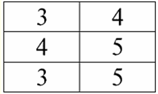
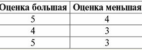

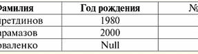

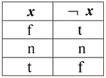

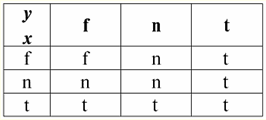
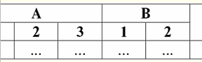
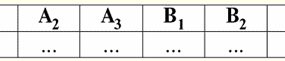
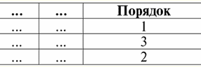
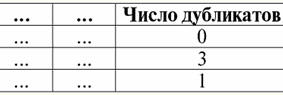
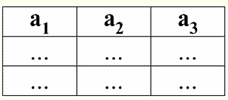

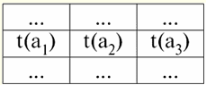


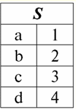
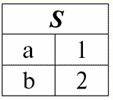

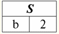
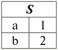

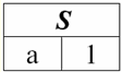
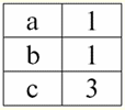

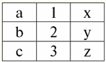


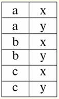


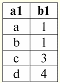
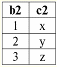


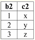


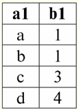
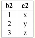


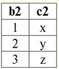

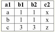
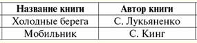
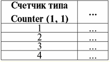


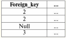
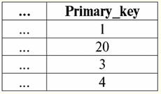

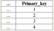
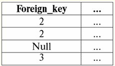
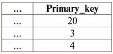
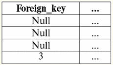

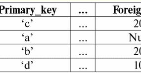


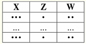


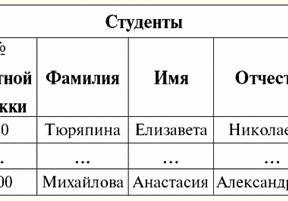
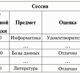
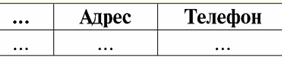

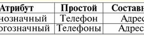
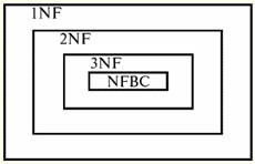

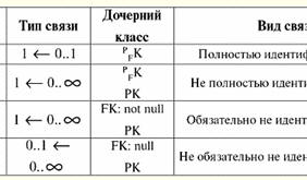

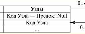

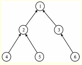
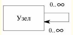


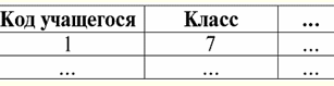
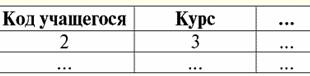

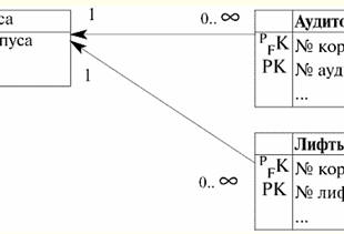

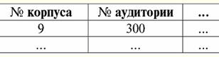


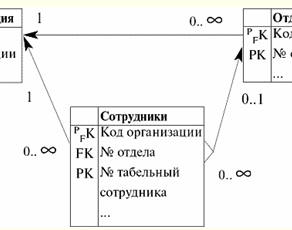
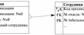
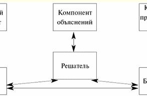
 See other articles Section