|
|


 Arabic
 Bengali
 Chinese
 English
 French
 German
 Hebrew
 Hindi
Hindi Italian
 Japanese
 Korean
 Malay
Malay Polish
 Portuguese
 Spanish
 Turkish
 Ukrainian
 Vietnamese
|
ENCYCLOPEDIA OF RADIO ELECTRONICS AND ELECTRICAL ENGINEERING Measure antenna parameters? Quite easy! Encyclopedia of radio electronics and electrical engineering
Encyclopedia of radio electronics and electrical engineering / Antennas. Measurements, adjustment, coordination Correctly defined antenna parameters in a radio reception system are the basis for the possibility of successfully receiving remote radio stations. But not always a radio amateur may have at hand the necessary tools for such measurements. In this article, the author proposes to use a simple method that produces quite acceptable results. Having suspended an outdoor wire antenna, a fan of radio reception on long and medium waves (LW and MW) often asks the question: what are its parameters? There are two main parameters - this is the loss resistance of the antenna-grounding system rp and the antenna's own capacitance relative to the same ground SA. The efficiency of the antenna system depends on these parameters, and, consequently, the possibility of receiving distant stations, feeding the receiving device with "free energy" of signals received from the air, tuning the antenna system to different frequencies, etc. Antenna measurements are "terra incognita" for most radio amateurs, and not just beginners. All known methods require a powerful high-frequency generator and a measuring bridge - equipment rarely found in radio amateurs. Often these two devices are combined to form a feeder or antenna ohmmeter (as they are called), used, for example, when tuning and adjusting antennas of transmitting radio centers [1]. A powerful RF generator is needed because the antenna, open to all winds, has a high voltage of various pickups, including from signals from other radio stations that interfere with measurements. In the proposed measurement method, the generator is not needed at all. We will measure the parameters of the antenna using signals from the air, since there are plenty of them there. Do I need to make a special device or stand for measurements? This is optional. Considering that the antennas are not changed every day, it will not be difficult to assemble simple measuring circuits right on the desktop or on the windowsill, without even using prototyping boards. Loss resistance measurement. You will need a ferrite rod from a magnetic antenna with a pair of coils, preferably LW and MW ranges, a variable resistor with a resistance of 0,47 ... ,1...0,5 MΩ). To identify received radio stations "by ear" it is useful to have high-impedance telephones. We assemble the device according to the scheme of Fig. 1 and, by moving the rod in the coil of the magnetic antenna, we tune in to the signal frequency of a powerful local radio station.
In this case, the variable resistor R1 must be set to the position of zero resistance (move the slider to the upper position according to the diagram). The moment of fine tuning the circuit in resonance with the frequency of the radio station will be marked by the maximum deviation of the meter needle and the highest volume in the phones. Phones connected in series with the voltmeter have practically no effect on its readings, at the same time, the volume is not too high. To increase it for the time of identifying the radio station, the voltmeter can be closed, switched to the lowest measurement limit, where its resistance is less, or a capacitor with a capacitance of the order of 0,05 ... capacitor, the sound may be somewhat distorted due to the inequality of the load of the detector at audio frequencies and at direct current). Noting the voltmeter readings (U1) and without changing the circuit settings, move the variable resistor R1 slider until the voltmeter readings are halved (U2). In this case, the resistance of the resistor will be equal to the loss resistance of the antenna system at a given frequency. The same measurements can be made at other frequencies. The resistance of the resistor is measured with an ohmmeter, disconnecting it from the measuring circuit. In the absence of an ohmmeter, it is necessary to equip the resistor with a pen with a sight and a scale, which should be calibrated in ohms using a standard instrument. Using the above methodology, it is possible to choose, for example, the best grounding option. In urban conditions, the following options are possible: water pipes, heating pipes, balcony railing fittings, etc., as well as various combinations of them. You should focus on the maximum received signal and the minimum loss resistance. In a country house, in addition to the "classic" grounding, it is recommended to try a water well or water pipes, a metal mesh fence, a galvanized sheet roof or any other massive metal object, even if it does not have contact with real earth. Antenna Capacitance Measurement. Instead of a variable resistor, now you need to turn on the KPI (of any type) with a maximum capacitance of 180 ... 510 pF. It is also desirable to have a capacitance meter with a measurement limit of tens to hundreds of picofarads. The author used a Master-S digital capacitance meter [2] kindly provided by its designer. If there is no capacitance meter, you must do the same as with a resistor - equip the KPI with a scale and calibrate it in picofarads. This can be done without devices, because the capacity is proportional to the area of the introduced part of the plates. Draw the shape of the rotor plate on graph paper (the larger, the more accurate the graduation), divide the drawing into sectors at 10 angular degrees and calculate the area of each sector and the entire plate S0 in cells. On fig. 2, the first sector with area S1 is shaded. At the first risk of the scale corresponding to it, it is necessary to set the capacity C1 \u1d CmaxS0 / SXNUMX, etc.
If the rotor plates have a semicircular shape (a direct capacitance capacitor), the scale turns out to be linear and then there is no need to make drawings and count the areas. For example, a KPI with a solid dielectric from a kit for children's creativity has a maximum capacitance of 180 pF. It is enough to divide the scale into 18 sectors of 10 degrees each, and put about divisions of 10, 20 pF, etc. Let the accuracy be low, for our purposes it is enough. Having calibrated the KPI, we assemble the installation according to the scheme of fig. 3.
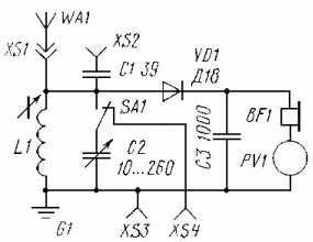
By connecting the antenna to the XS1 jack and turning off the KPI with the SA1 switch, we tune the circuit formed by the antenna capacitance and the L1 coil to the frequency of the radio station. Without touching the coil anymore, we switch the antenna to the XS2 socket and connect the capacitor C2 (our KPI) to the circuit with the SA1 switch. We tune in to the same frequency again, now with the help of C2. We determine its capacitance Sk on a scale or using a capacitance meter connected to the sockets XS3, XS4 (switching SA1 to the position shown in the diagram for this). It remains to find the capacitance of the SA antenna by the formula SA = C2(1 + sqrt(1 + 4C1/C2))/2. The meaning of our manipulations is as follows: when we connected the antenna through the coupling capacitor C1, the total capacitance of the circuit became smaller, and in order to restore it, we had to add capacitance C2. You yourself can derive the above formula based on the equality of the capacitance of the CA antenna (in the first case) and the complex contour capacitance C2 + CAC1 / (CA + C1) in the second case. To improve the accuracy of measurements, it is desirable to choose a smaller capacitance of the coupling capacitor, within 15 ... 50 pF. If the capacitance of the coupling capacitor is much less than the capacitance of the antenna, then the calculation formula is simplified: SA = C2 + C1. Experiment and discussion. The author measured the parameters of an antenna of this type available at the dacha: a PEL 0,7 wire 15 m long, which is stretched to the roof ridge and away from the house to a neighboring tree. The best "grounding" (counterweight) was a water heater isolated from the ground with a small network of pipes and local heating batteries. All measurements were carried out in the MW range using a standard MW coil of a magnetic antenna from a transistor receiver. If there was not enough inductance to tune at the low-frequency edge of the range, another ferrite rod was placed next to the magnetic antenna, parallel to the first.
The measurement results are summarized in the table. They need a little comment. First of all, it is striking that at different frequencies both the loss resistance and the capacitance of the antenna are different. These are not measurement errors at all. Consider first the frequency dependence of the capacitance. If the antenna wire did not also have some inductance LA, the capacitance values would be the same. The wire inductance is in series with the antenna capacitance, as seen from the antenna circuit equivalent circuit shown in Fig. 4.
The influence of inductance is stronger at high frequencies, where the inductive reactance increases and partially compensates for the capacitive reactance. As a result, the total reactance of the antenna decreases and the measured capacitance becomes larger. The antenna has a natural frequency f0 - the resonant frequency of the LACA circuit, at which the reactance vanishes, and the measured capacitance value tends to infinity. The natural wavelength of the Lambda0 antenna corresponding to this frequency is approximately equal to four times the length of the antenna wire and usually falls within the HF range. The natural frequency can be calculated from capacitance measurements at two arbitrary frequencies, but the formulas are too complicated. For his antenna, the author received CA = 85 pF. LA = 25 μH and f0 - about 3,5 MHz. For approximate estimates, we can assume that each meter of antenna wire (together with the reduction) introduces an inductance of about 1 ... 1,5 μH and a capacitance of about 6 pF. The loss resistance with a sufficiently good quality coil L1 consists mainly of the ground resistance. It, in turn, is calculated according to the empirical (obtained on the basis of experimental data) formula of M.V. Shuleikin [3]: rp = А*Lambda/Lambda0. Here A is a constant coefficient depending on the quality of the grounding, with a dimension in ohms. For good grounds, A is units and even fractions of an ohm. As you can see, the loss resistance increases with increasing wavelength (lowering the frequency), which was confirmed by the data in the table. The frequency dependence of the loss resistance was discovered at the beginning of the last century, but the author did not find a detailed explanation of this effect in the literature. In this regard, many of the data obtained by radio amateurs when measuring the parameters of their antennas can be very useful. Literature
Author: V.Polyakov, Moscow
The existence of an entropy rule for quantum entanglement has been proven
09.05.2024 Mini air conditioner Sony Reon Pocket 5
09.05.2024 Energy from space for Starship
08.05.2024
▪ Supersteel modeled after human bone ▪ Thermal power plant on vegetable oil ▪ Alarm signal - in every house ▪ Small glasses for a big picture
▪ section of the site Calls and audio simulators. Article selection ▪ Article Internal Medicine. Crib ▪ article Where and when was a concept book consisting only of blank pages sold? Detailed answer ▪ Knikus article. Legends, cultivation, methods of application ▪ article Electronic phase meter. Encyclopedia of radio electronics and electrical engineering
Home page | Library | Articles | Website map | Site Reviews
www.diagram.com.ua |


 Leave your comment on this article: