|
|


 Arabic
 Bengali
 Chinese
 English
 French
 German
 Hebrew
 Hindi
Hindi Italian
 Japanese
 Korean
 Malay
Malay Polish
 Portuguese
 Spanish
 Turkish
 Ukrainian
 Vietnamese
|
Lecture notes, cheat sheets
General theory of statistics. Lecture summary: briefly, the most important
Directory / Lecture notes, cheat sheets Table of contents
LECTURE No. 1. Statistics as a science 1. The subject and method of statistics as a social science Statistics - an independent social science, which has its own subject and methods of research, which arose from the needs of social life. Statistics is a science that studies the quantitative side of all socio-economic phenomena. The term "statistics" comes from the Latin word "status", which means "position, order". For the first time it was used by the German scientist G. Achenwal (1719-1772). The main task of statistics is to mathematically correctly describe the collected information. Statistics can be called a special section of mathematics that describes one or another side of human life. Statistics uses a variety of mathematical methods and techniques so that a person can analyze a particular problem. Statistics can provide invaluable assistance to any leader in any enterprise, if you know how to use it correctly. To date, the term "statistics" is used in three meanings: 1) a special branch of practical activity of people aimed at collecting, processing and analyzing data that characterize the socio-economic development of the country, its regions, individual sectors of the economy or enterprises; 2) a science that develops theoretical provisions and methods used in statistical practice; 3) statistics - statistical data presented in the reports of enterprises, sectors of the economy, as well as data published in collections, various directories, bulletins, etc. Statistics object - phenomena and processes of the socio-economic life of society, in which the socio-economic relations of people are displayed and find their expression. The general theory of statistics is the methodological basis, the core of all sectoral statistics. It develops general principles and methods for the statistical study of social phenomena and is the most general category of statistics. The tasks of economic statistics are the development and analysis of synthetic indicators that reflect the state of the national economy, the relationship of industries, the peculiarities of the distribution of productive forces, the availability of material, labor and financial resources. Social statistics develops a system of indicators to characterize the way of life of the population and various aspects of social relations. Statistics - social science, which is engaged in the collection of information of a different nature, its ordering, comparison, analysis and interpretation (explanation). It has the following distinctive features: 1) studies the quantitative side of social phenomena. This side of the phenomenon represents its magnitude, size, volume and has a numerical dimension; 2) explores the qualitative side of mass phenomena. The provided side of the phenomenon expresses its specificity, the internal feature that distinguishes it from other phenomena. The qualitative and quantitative sides of a phenomenon always exist together, form one single whole. All social phenomena and events take place in time and space, and in relation to any of them it is always possible to determine at what time it arose and where it develops. Thus, statistics studies phenomena in specific conditions of place and time. The phenomena and processes of social life comprehended by statistics are in constant change and development. Based on the collection, processing and analysis of mass data on changes in the studied phenomena and processes, a statistical regularity is revealed. Statistical regularities manifest the actions of social laws that determine the existence and development of socio-economic relations in society. The subject of statistics is the study of social phenomena, the dynamics and direction of their development. With the help of statistical indicators, statistics establishes the quantitative side of a social phenomenon, observes the patterns of the transition of quantity into quality using the example of a given social phenomenon. On the basis of the observations provided, statistics analyzes the data obtained in specific conditions of place and time. Statistics is engaged in the study of socio-economic phenomena and processes that are massive, and also studies the many factors that determine them. To derive and confirm their theoretical laws, most of the social sciences use statistics. The conclusions formed on statistical studies are used by economics, history, sociology, political science and many other humanities. Statistics is also necessary for the social sciences to confirm their theoretical basis, and its practical role is very great. Neither large enterprises nor serious industries, when developing a strategy for the economic and social development of an object, can do without the analysis of statistical data. For this, special analytical departments and services are organized at enterprises and industries, attracting specialists who have completed professional training in this discipline. Statistics, like any other science, has a certain set of methods for studying its subject. Methods of statistics are chosen depending on the phenomenon under study and the specific subject of research (relationships, patterns or development). Methods in statistics are formed in the aggregate from the developed and applied specific methods and techniques for the study of social phenomena. These include observation, summary and grouping of data, calculation of generalizing indicators based on special methods (method of averages, indices, etc.). In this regard, there are three stages of working with statistical data: 1) collection is a mass scientifically organized observation, through which primary information about individual facts (units) of the phenomenon under study is obtained. This statistical accounting of a large number or all of the units that make up the phenomenon under study is the information base for statistical generalizations, for drawing conclusions about the phenomenon or process under study; 2) grouping and summary. These data are understood as the distribution of a set of facts (units) into homogeneous groups and subgroups, the final count for each group and subgroup, and the presentation of the results in the form of a statistical table; 3) processing and analysis. Statistical analysis concludes the stage of statistical research. It contains the processing of statistical data that were obtained during the summary, the interpretation of the results obtained in order to obtain objective conclusions about the state of the phenomenon under study and about the patterns of its development. In the process of statistical analysis, the structure, dynamics and interconnection of social phenomena and processes are studied. The main stages of statistical analysis are: 1) assertion of facts and establishment of their assessment; 2) identification of characteristic features and causes of the phenomenon; 3) comparison of the phenomenon with normative, planned and other phenomena, which are taken as the basis for comparison; 4) formulation of conclusions, forecasts, assumptions and hypotheses; 5) statistical verification of the proposed assumptions (hypotheses). 2. Theoretical foundations and basic concepts of statistics For statistical methodology, the theoretical basis is the dialectical materialistic understanding of the laws of the process of development of society. As a result, statistics often uses such categories as quantity and quality, necessity and chance, regularity, causality, etc. The main provisions of statistics are based on the laws of social and economic theory, since they consider the patterns of development of social phenomena, determine their significance, causes and consequences for the life of society. On the other hand, the laws of many social sciences are created on the basis of statistics and patterns identified through statistical analysis, so we can say that the relationship between statistics and other social sciences is endless and continuous. Statistics establishes the laws of the social sciences, and they, in turn, correct the provisions of statistics. The theoretical basis of statistics is also closely related to mathematics, since it is necessary to use mathematical indicators, laws and methods to measure, compare and analyze quantitative characteristics. A deep study of the dynamics of a phenomenon, its change in time, as well as its relationship with other phenomena is impossible without the use of higher mathematics and mathematical analysis. Very often, a statistical study is based on a developed mathematical model of a phenomenon. Such a model theoretically reflects the quantitative ratios of the phenomenon under study. If it is available, the task of statistics is to numerically determine the parameters included in the model. When assessing the financial condition of an enterprise, A. Altman's scoring model is often used, where the level of bankruptcy Z is calculated using the following formula: Z=1,2x1 + 1,4x2 + 3,3x3 + 0,6x4 + 10,0x5, where x1 - the ratio of reverse capital to the amount of assets of the company; x2 - the ratio of undistributed income to the amount of assets; x3 - the ratio of operating income to the amount of assets; x4 - the ratio of the market value of the company's shares to the total amount of debt; x5 - the ratio of the amount of sales to the amount of assets. According to A. Altman, if Z < 2,675, the firm is threatened with bankruptcy, and if Z > 2,675, the financial position of the firm is beyond fear. To get this estimate, it is necessary to substitute the unknown x into the formula1,x2,x3,x4 and x5, which are certain indicators of balance lines. Particularly widespread in statistical science are such areas of mathematics as probability theory and mathematical statistics. In statistics, operations are used that are directly calculated using the rules of probability theory. This is a selective observation method. The main of these rules is a series of theorems expressing the law of large numbers. The essence of this law lies in the disappearance of the element of randomness in the summary indicator, with which individual characteristics are associated, as more and more of them are combined in it. Mathematical statistics is also closely related to probability theory. The tasks considered in it can be classified into three categories: distribution (set structure), connections (between features), dynamics (change over time). The analysis of variational series is widely used, the forecasting of the development of phenomena is carried out with the help of extrapolations. Causal relationships of phenomena and processes are introduced using correlation and regression analysis. Finally, statistical science is indebted to mathematical statistics for its most important categories and concepts, such as totality, variation, sign, regularity. The statistical totality belongs to the main categories of statistics and is the object of statistical research, which is understood as a systematic scientifically based collection of information about the socio-economic phenomena of public life and analysis of the data obtained. In order to carry out a statistical study, a scientifically reasoned information base is needed. Such an information base is a statistical set - a set of socio-economic objects or phenomena of social life, united by a common connection, a qualitative basis, but differing from each other in some characteristics (for example, a set of households, families, firms, etc.). From the point of view of statistical methodology, a statistical population is a set of units that have such characteristics as homogeneity, mass character, a certain integrity, the presence of variation, and the interdependence of the state of individual units. Thus, the statistical population consists of individual units. An object, a person, a fact, a process can be a unit of the totality. The unit of the population is the primary element and the carrier of its main features. The element of the population for which the necessary data for a statistical study is collected is called the unit of observation. The number of units in the population is called the size of the population. The statistical aggregate can be the population during the census, enterprises, cities, employees of the company. The choice of a statistical population and its units depends on the specific conditions and nature of the socio-economic phenomenon or process being studied. The mass nature of the units of the population is closely related to its completeness. Completeness is ensured by the coverage of units of the statistical population under study. For example, the researcher must draw a conclusion about the development of banking. Therefore, he needs to collect information on all banks operating in the region. Since any set has a rather complex character, then completeness should be understood as the coverage of the set of the most diverse features of the set, which reliably and essentially describe the phenomenon under study. If, for example, financial results are not taken into account in the process of monitoring banks, then it is impossible to draw final conclusions about the development of the banking system. In addition, completeness suggests the study of the characteristics of units of the population for the longest possible periods. Fairly complete data are, as a rule, massive and exhaustive. The socio-economic phenomena studied in practice are very diverse, therefore it is difficult and sometimes even impossible to cover all phenomena. The researcher is forced to study only a part of the statistical population, and draw conclusions for the entire population. In such situations, the most important requirement is the reasonable selection of the part of the population for which the characteristics are studied. This part should display the main properties, phenomena and be typical. In reality, several aggregates can simultaneously interact in the phenomena and processes under study. In these situations, the object of study is found in such a way as to clearly distinguish the studied populations. A sign of a unit of an aggregate is its characteristic feature, a specific property, feature, quality that can be observed and measured. The population studied in time or space must be comparable. Consequently, the requirements of their comparability and uniformity are imposed on the characteristics of the population units. For this, it is necessary to use, for example, uniform cost estimates. In order to qualitatively investigate the totality, the most significant or interrelated features are studied. The number of features characterizing the population unit should not be excessive. This complicates the collection of data and the processing of results. The characteristics of units of the statistical population must be combined so that they complement each other and have interdependence. The requirement of homogeneity of the statistical population means the choice of the criterion according to which one or another unit belongs to the population under study. For example, if the initiative of young voters is studied, then it is necessary to establish age limits for such voters in order to exclude people of the older generation. It is possible to limit such a population to representatives of rural areas or, for example, students. The presence of variation in the units of the population means that their characteristics can receive all kinds of values or modifications in some units of the population. In this regard, such signs are called varying, and individual values or modifications are called variants. Signs are divided into attributive and quantitative. A sign is called attributive or qualitative if it is expressed by a semantic concept, for example, a person's gender or his belonging to a particular social group. Internally, they are divided into nominal and ordinal. An attribute is called quantitative if it is expressed as a number. According to the nature of variation, quantitative signs are divided into discrete and continuous. An example of a discrete feature is the number of people in a family. In the form of integers, as a rule, variants of discrete features are expressed. Continuous features include, for example, age, salary, length of service, etc. According to the method of measurement, signs are divided into primary (accounted) and secondary (calculated). Primary (accounted for) express the unit of the population as a whole, i.e., absolute values. Secondary (calculated) are not directly measured, but calculated (cost, productivity). Primary features underlie the observation of a statistical population, while secondary features are determined in the process of data processing and analysis and represent the ratio of primary features. In relation to the characterized object, signs are divided into direct and indirect. Direct signs are properties that are directly inherent in the object that is characterized (volume of production, age of a person). Indirect signs are properties that are characteristic not of the object itself, but of other aggregates related to the object or included in it. In relation to time, instantaneous and interval signs are distinguished. Momentary signs characterize the object under study at some point in time, established by the plan of statistical research. Interval signs characterize the results of processes. Their values can only occur over a time interval. In addition to signs, the state of the object under study or the statistical population is characterized by indicators. Indicators - one of the main concepts of statistics, which is a generalized quantitative assessment of socio-economic processes and phenomena. According to the target functions, statistical indicators are divided into accounting and evaluation and analytical. Accounting and estimated indicators - this is a statistical characteristic of the magnitude of socio-economic phenomena in the established conditions of place and time, i.e. they reflect the volume of distribution in space or the levels reached at a certain time. Analytical indicators are used to analyze the data of the studied statistical population and characterize the specifics of the development of the studied phenomena. As analytical indicators in statistics, relative, average values, indicators of variation and dynamics, indicators of communication are used. The totality of statistical indicators reflecting the relationships that exist between phenomena forms a system of statistical indicators. In general, indicators and signs fully characterize and comprehensively describe the statistical population, allowing the researcher to conduct a complete study of the phenomena and processes of the life of human society, which is one of the goals of statistical science. The central category of statistics is statistical regularity. Regularity is generally understood as a detectable causal relationship between phenomena, the sequence and repetition of individual features that characterize the phenomenon. In statistics, regularity is understood as the quantitative regularity of changes in space and time of mass phenomena and processes of social life as a result of the action of objective laws. Consequently, the statistical regularity is characteristic not of individual units of the population, but of the entire population as a whole and is expressed only with a sufficiently large number of observations. Thus, the statistical regularity reveals itself as an average, social, mass regularity in the mutual cancellation of individual deviations of the values of signs in one direction or another. So, the manifestation of a statistical regularity gives us the opportunity to present a general picture of the phenomenon, to study the trend of its development, excluding random, individual deviations. 3. Modern organization of statistics in the Russian Federation Statistics plays an important role in managing the economic and social development of the country, since the correctness of any management conclusion largely depends on the information on the basis of which it is made. Only accurate, reliable and correctly analyzed data should be taken into account at high levels of management. The study of the economic and social development of the country, individual regions, industries, firms, enterprises is carried out by specially formed bodies that make up the statistical service. In the Russian Federation, the functions of the statistical service are performed by departmental statistics bodies and state statistics bodies. The highest governing body for statistics is the State Statistics Committee of the Russian Federation. It solves the main tasks currently facing Russian statistics, provides a holistic methodological basis for accounting, consolidates and analyzes the information received, summarizes the data, and publishes the results of its activities. The State Committee on Statistics of the Russian Federation (Goskomstat of Russia) was established in accordance with the Decree of the President of the Russian Federation of December 6, 1999 No. 1600 "On the transformation of the Russian Statistical Agency into the State Committee of the Russian Federation on Statistics". The State Statistics Committee of the Russian Federation is a federal executive body responsible for intersectoral coordination and functional regulation in the field of state statistics. The State Committee on Statistics of the Russian Federation performs the following functions: 1) carries out the collection, processing, protection and storage of statistical information, observance of state and commercial secrets, the necessary confidentiality of data; 2) ensures the functioning of the Unified State Register of Enterprises and Organizations (EGRPO) on the basis of accounting for all economic entities on the territory of the Russian Federation with the assignment of identification codes to them, based on the all-Russian classifiers of technical, economic and social information; 3) develop a scientifically based statistical methodology that meets the needs of society at the present stage, as well as international standards; 4) checks the compliance of all legal and other economic entities with the laws of the Russian Federation, decisions of the President of the Russian Federation, the Government of the Russian Federation on statistics; 5) issues resolutions and instructions on statistical issues that are binding on all legal and other economic entities located on the territory of the Russian Federation. The set of methods of statistical indicators, methods and forms of collecting and processing statistical data adopted by the State Statistics Committee of Russia are the official statistical standards of the Russian Federation. The Goskomstat of Russia in its main activities is guided by federal statistical programs, which are formed taking into account the proposals of the federal executive and legislative authorities, state authorities of the constituent entities of the Russian Federation, scientific and other organizations and are approved by the Goskomstat of Russia in agreement with the Government of the Russian Federation. The main tasks of the statistical bodies of the country are to ensure the publicity and accessibility of general (not individual) information, as well as guarantee the reliability, truthfulness and accuracy of the data taken into account. In addition, the tasks of the State Statistics Committee of Russia are: 1) submission of official statistical information to the President of the Russian Federation, the Federal Assembly of the Russian Federation, the Government of the Russian Federation, federal executive authorities, the public, as well as international organizations; 2) development of a scientifically proven statistical methodology that meets the needs of society at the present stage, as well as international standards; 3) coordination of the statistical activities of federal executive authorities and executive authorities of the constituent entities of the Russian Federation, provision of conditions for the application by these authorities of official statistical standards when they conduct sectoral (departmental) statistical observations; 4) development and analysis of economic and statistical information, preparation of the necessary balance calculations and national accounts; 5) guaranteeing complete and scientifically based statistical information; 6) providing all users with equal access to open statistical information by distributing official reports on the socio-economic situation of the Russian Federation, constituent entities of the Russian Federation, industries and sectors of the economy, publishing statistical collections and other statistical materials. As a result of reforming the economy of the Russian Federation, the structure of statistical bodies has also changed. Local district statistical registries have been abolished and inter-district statistical departments have been formed, which are representative offices of territorial statistical bodies. The organization of statistical bodies in Russia is now at the stage of reform. As noted above, at present, statistical science in Russia is undergoing some changes. The main areas in which reforms should be made can be noted: 1) it is necessary to comply with the basic law of statistical accounting - publicity and availability of information while maintaining the confidentiality of individual indicators (trade secrets); 2) it is necessary to reform the methodological and organizational foundations of statistics: a change in the general tasks and principles of economic management leads to a change in the theoretical provisions of science; 3) the transition to market statistics gives rise to the need to improve the system for collecting and processing information by introducing such forms of observation as qualifications, registers (registries), censuses, etc.; 4) it is necessary to change (improve) the methodology for calculating some statistical indicators that characterize the state of the economy of the Russian Federation, while taking into account international standards, foreign experience in statistical accounting, it is necessary to systematize all indicators and put them in order corresponding to the issues and requirements of the time, taking into account the system of national accounts (SNA); 5) it is necessary to ensure the relationship of statistical indicators characterizing the level of development of the country's public life; 6) trends in computerization should be taken into account. In the course of reforming statistical science, a unified information base (system) should be created, which will include the information bases of all statistical bodies that are at a lower level of the hierarchical ladder of the organization of state statistics. Thus, structural changes are still taking place in Russia that affect all spheres of the country's public life. Since statistics is directly related to almost all of these areas, the reform process has not bypassed it either. At present, a lot of work has been done to organize the work of statistical bodies, but it has not yet been completed, and much attention remains to be paid to improving this information institution, which is very significant for the state. Along with state statistical services, there is departmental statistics, which is maintained in ministries, departments, enterprises, associations and firms of various sectors of the economy. Departmental statistics is engaged in the collection, processing and analysis of statistical information. This information is necessary for making management decisions, for planning the activities of an organization or authority. In small businesses, this work is usually done either by the chief accountant or directly by the manager himself. At large enterprises that have their own regional structure branched out or have a large number of employees, entire departments or departments are involved in the processing and analysis of statistical information. Such work involves specialists in the field of statistics, mathematics, accounting and economic analysis, managers and technologists. Such a team, armed with modern computer technology, based on the methodology proposed by the theory of statistics, and using modern methods of analysis, helps to build effective business development strategies, as well as effectively shape the activities of public authorities. It is impossible to manage complex social and economic systems without complete, reliable and timely statistical information. Thus, the bodies of state and departmental statistics face a very significant task of theoretical substantiation of the volume and composition of statistical information, corresponding to modern conditions of economic development, contributing to rationalization in the system of accounting and statistics and minimizing the costs of performing this function. LECTURE No. 2. Statistical observation 1. The concept of statistical observation, the stages of its implementation A deep comprehensive study of any economic or social process involves measuring its quantitative side and characterizing its qualitative essence, place, role and relationships in the general system of social relations. Before you start using statistical methods for studying the phenomena and processes of social life, you need to have at your disposal an exhaustive information base that fully and reliably describes the object of study. The process of statistical research involves the following steps: 1) collection of information on statistics (statistical observation) and its primary processing; 2) grouping and subsequent processing of data obtained as a result of statistical observation, based on their summary and grouping; 3) generalization and analysis of the results of processing statistical materials, formulation of conclusions and recommendations based on the results of the entire statistical study. Therefore, statistical observation is the first and the initial stage of the statistical study. Statistical observation - the process of collecting primary data on various phenomena of social and economic life. This means that statistical observation should be organized as planned, massive and systematic. The regularity of statistical observation lies in the fact that it is carried out according to a specially developed plan, which contains issues related to the organization and technique of collecting statistical information, monitoring its reliability and quality, and presenting the final materials. The mass nature of statistical observation is ensured by the most complete range of all cases of manifestation of the phenomenon or process under study, i.e., quantitative and qualitative characteristics are measured and recorded not by individual units of the population under study, but by the entire mass of units of the population in the process of statistical observation. The systematic nature of statistical observation should not be spontaneous. The work associated with such monitoring should be carried out either continuously or regularly, at regular intervals. The process of preparing a statistical observation involves setting the goal and object of observation, choosing the unit of observation, the composition of features to be recorded. To collect data, it is necessary to develop forms of documents and choose the means and methods for obtaining them. Consequently, statistical observation is laborious and painstaking work that requires the involvement of qualified personnel, its comprehensive organization, planning, preparation and implementation. 2. Types and methods of statistical observation Statistical observation is a process that, from the point of view of its organization, can have a variety of methods, forms and types of conduct. The task of the general theory of statistics is to determine the essence of the methods, forms and types of observation in order to decide where, when and what methods of observation will be applied. Statistical observations have two main groups: 1) coverage of population units; 2) time of registration of facts. According to the level of coverage of the studied population, statistical observation is divided into two types: continuous and non-continuous. Continuous (complete) observation refers to the coverage of all units of the studied population. Continuous observation provides completeness of information about the studied phenomena and processes. This type of observation is associated with high costs of labor and material resources. The collection and processing of the entire amount of necessary information requires considerable time, so the need for operational information is not satisfied. Often continuous observation is impossible at all (for example, when the population under study is too large or there is no possibility of obtaining information about all units of the population). As a result, inconsistent observations are made. Under non-continuous observation is understood only the coverage of a certain part of the studied population. When conducting a non-continuous observation, it is necessary to determine in advance which part of the population under study will be subjected to observation and what criterion will be used as the basis for the sample. The advantage of organizing a non-continuous observation is that it is carried out in a short time, is associated with the lowest labor and material costs, and the information obtained is of an operational nature. There are several types of discontinuous observation: selective; observation of the main array; monographic. Selective observation is understood as a part of the units of the studied population, selected by the method of random selection. With the right organization, sample observation produces fairly accurate results that can be extended with conditional probability to the entire population. The method of momentary observations is called selective observation, which involves the selection of not only units of the population under study (sampling in space), but also the points in time at which the registration of signs is carried out (sampling in time). Observation of the main array is the coverage of the survey of certain, most significant features of the units of the population. With such an observation, the largest units of the population are taken into account, and the most significant features for this study are recorded. For example, 15-20% of large credit institutions are surveyed, while the content of their investment portfolios is recorded. Monographic observation is characterized by a comprehensive and complete study of only some units of the population that have some special characteristics or represent some new phenomenon. The purpose of such observation is to identify existing or only emerging trends in the development of a given process or phenomenon. In a monographic survey, individual units of the population are subjected to a detailed study, which allows us to note very important dependencies and proportions that we cannot find with other, less detailed observations. Statistical-monographic surveys are often used in medicine, when examining family budgets, etc. It is important to note that monographic surveys are closely related to continuous and selective surveys. Firstly, data from mass surveys are needed to select a criterion for selecting population units for non-continuous and monographic observation. Secondly, monographic observation makes it possible to identify the characteristic features and essential features of the object of study, to clarify the structure of the studied population. The findings can be used as the basis for organizing a new mass survey. According to the time of registration of facts, observation can be continuous and discontinuous. Discontinuous monitoring, in turn, includes periodic and one-time. Continuous (current) observation is realized by continuous registration of facts as they become available. With such an observation, all changes in the processes and phenomena under study are traced, which makes it possible to monitor its dynamics. For example, registry offices register deaths, births, and marriages continuously. The enterprises maintain current records of the release of materials from the warehouse, production, etc. Discontinuous observation is carried out either systematically, at fixed intervals (periodic observation), or once and irregularly as necessary (one-time observation). Periodic observations are usually based on a similar program and tools so that the results of such studies can be comparable. Examples of periodic observation can be a population census conducted at fairly long intervals, and all forms of statistical observations that are annual, semi-annual, quarterly, monthly. The specificity of a one-time observation is that the facts are recorded not in connection with their occurrence, but according to their state or presence at a certain moment or over a period of time. Quantitative measurement of signs of a phenomenon or process occurs at the time of the survey, and re-registration of signs may not be carried out at all or the timing of its implementation is not predetermined. An example of a one-time observation is a one-time survey of the state of housing construction, which was conducted in 2000. Along with the types of statistical observation, the general theory of statistics considers methods for obtaining statistical information, the most important of which are the documentary method of observation; method of direct observation; interview. Documentary observation is based on the use of data from various documents, such as accounting registers, as a source of information. Considering that, as a rule, high requirements are imposed on filling out such documents, the data reflected in them are of the most reliable nature and can serve as a high-quality source material for analysis. Direct observation is carried out by registering the facts personally established by the registrars as a result of inspection, measurement, and counting the signs of the phenomenon under study. In this way, prices for goods and services are recorded, measurements of working hours are made, an inventory of stock balances, etc. The survey is based on obtaining data from respondents (survey participants). The survey is used in cases where observation by other methods cannot be carried out. This type of observation is typical for conducting various sociological surveys and public opinion polls. Statistical information can be obtained by different types of surveys: expeditionary; correspondent; questionnaire; secret. Expeditionary (oral) survey is carried out by specially trained workers (registrators), who record the answers of respondents in the observation forms. The form is a form of a document in which it is necessary to fill in the fields for answers. The correspondent method assumes that, on a voluntary basis, the respondent staff reports information directly to the monitoring body. The disadvantage of this method is that it is difficult to verify the correctness of the received information. In the questionnaire method, respondents fill out questionnaires (questionnaires) voluntarily and mostly anonymously. Since this method of obtaining information is not reliable, it is used in those studies where high accuracy of the results is not required. In some situations, approximate results are sufficient, which capture only the trend and record the emergence of new facts and phenomena. The secret method involves the submission of information to the bodies conducting monitoring, in secret. In this way, acts of civil status are registered - marriages, divorces, deaths, births, etc. In addition to the types and methods of statistical observation, the theory of statistics also considers the forms of statistical observation: reporting; specially organized statistical observation; registers. Statistical reporting - the main form of statistical observation, which is characterized by the fact that statistical authorities receive information about the phenomena under study in the form of special documents submitted by enterprises and organizations within a certain time frame and in the prescribed form. The forms of statistical reporting themselves, the methods of collecting and processing statistical data, the methodology of statistical indicators established by the State Statistics Committee of Russia are the official statistical standards of the Russian Federation and are mandatory for all subjects of public relations. Statistical reporting is divided into specialized and standard. The composition of indicators of standard reporting is the same for all enterprises and organizations, while the composition of indicators of specialized reporting depends on the specifics of individual sectors of the economy and areas of activity. According to the timing of submission, statistical reporting is daily, weekly, ten-day, two-weekly, monthly, quarterly, semi-annual and annual. Statistical reporting can be transmitted by telephone, via communication channels, on electronic media with mandatory subsequent submission on paper, certified by the signature of responsible persons. Specially organized statistical observation is a collection of information organized by statistical authorities, either to study phenomena that are not covered by reporting, or to study reporting data in more depth, verify and refine them. Various kinds of censuses, one-time surveys are specially organized observations. Registers - this is a form of observation in which the facts of the state of individual units of the population are continuously recorded. Observing a unit of the population, it is assumed that the processes taking place there have a beginning, a long-term continuation and an end. In the register, each unit of observation is characterized by a set of indicators. All indicators are stored until the observation unit is in the register and has not ended its existence. Some indicators remain unchanged as long as the unit of observation is in the register, others may change from time to time. An example of such a register is the unified state register of enterprises and organizations (USRE). All work on its maintenance is carried out by the State Statistics Committee of Russia. So, the choice of types, methods and forms of statistical observation depends on a number of factors, the main of which are the goals and objectives of observation, the specifics of the observed object, the urgency of presenting results, the availability of trained personnel, the possibility of using technical means of collecting and processing data. 3. Program and methodological issues of statistical observation One of the most important tasks that must be solved when preparing a statistical observation is the definition of the purpose, object and unit of observation. The goal of almost any statistical observation is to obtain reliable information about the phenomena and processes of social life in order to identify the interrelationships of factors, assess the scale of the phenomenon and the patterns of its development. Proceeding from the tasks of observation, its program and forms of organization are determined. In addition to the goal, it is necessary to establish the object of observation, that is, to determine what exactly is to be observed. The object of observation is the totality of social phenomena or processes to be studied. The object of observation can be a set of institutions (credit, educational, etc.), the population, physical objects of the building, transport, equipment). When establishing the object of observation, it is important to strictly and accurately determine the boundaries of the population under study. To do this, it is necessary to clearly establish the essential features by which it is determined whether to include an object in the aggregate or not. For example, before conducting a survey of medical institutions for the provision of modern equipment, it is necessary to determine the category, departmental and territorial affiliation of the clinics to be surveyed. When defining the object of observation, it is necessary to specify the unit of observation and the unit of the population. The unit of observation is a constituent element of the object of observation, which is a source of information. Depending on the specific tasks of statistical observation, the units of observation can be a household or a person, such as a student, an agricultural enterprise or a factory. Population unit - this is the so-called constituent element of the object of observation, from which information is received about the unit of observation, i.e., which serves as the basis for counting and has features that are subject to registration in the process of observation. For example, in a census of forest plantations, the unit of the population will be a tree, since it has characteristics that are subject to registration (age, species composition, etc.), while the forestry itself, in which the survey is conducted, acts as the unit of observation. Observation units are called reporting units if they submit statistical reports to the statistical authorities. Each phenomenon or process of social life has many features that characterize them. It is impossible to obtain information about all the features, and not all of them are of interest to the researcher. When preparing an observation, it is necessary to decide which signs will be subject to registration in accordance with the goals and objectives of the observation. To determine the composition of the registered signs, an observation program is developed. The program of statistical observation is a set of questions, the answers to which in the process of observation should form statistical information. The development of an observation program is a very important and responsible task, and the success of the observation depends on how correctly it is carried out. When developing an observation program, a number of requirements for it must be taken into account. Let's list the main ones. 1. The program should, if possible, contain only those features that are necessary and whose values will be used for further analysis or for control purposes. While striving for the completeness of information that ensures the receipt of benign materials, it is still necessary to limit the amount of information collected in order to obtain, albeit small, but reliable material for analysis. 2. The questions of the program must be formulated clearly enough, extremely clearly, in order to exclude their incorrect interpretation and prevent the distortion of the meaning of the information being collected. 3. When developing an observation program, it is desirable to build a logical sequence of questions. Questions of the same type or signs that characterize any one side of the phenomenon should be combined into one section. 4. It is important that the monitoring program contains control questions for checking and correcting the recorded information. To carry out the observation, you need your own tools - forms and instructions. statistical form - This is a special document of a single sample, in which answers to the questions of the program are recorded. Depending on the specific content of the observation being carried out, the form may be called a form of statistical reporting, a census or questionnaire, a map, a card, a questionnaire or a form. There are two types of forms - card and list. The card form (or individual form) is intended to reflect information about one unit of the statistical population, and the list form contains information about several units of the population. The integral and obligatory elements of the statistical form are the title, address and content parts. The title part indicates the name of the statistical observation and the body that approved this form, the terms for submitting the form and some other information. The address part contains the details of the reporting unit of observation. The main, content part of the form is usually drawn up in the form of a table, which in a convenient form contains the name, codes and values of indicators. The statistical form is filled in according to the instructions. The instruction contains instructions on the procedure for conducting observations and methodological instructions and explanations for filling out the form. Depending on the complexity of the surveillance program, the instruction is either published as a brochure or placed on the back of the form. In addition, for the necessary clarifications, you can contact the specialists responsible for conducting the observation, the bodies that conduct it. When organizing statistical observation, it is necessary to resolve the issue of the time of observation and the place of its conduct. The choice of the observation site depends on the purpose of the observation. The choice of observation time is associated with the determination of a critical moment (date) or time interval and the determination of the period (period) of observation. The critical moment of statistical observation is the point in time to which the information recorded in the process of observation is timed. The observation period determines the period during which the registration of information about the phenomenon under study should be carried out, that is, the time interval during which the forms are filled out. Usually, the observation period should not be too far from the critical moment of observation in order to reproduce the state of the object at that moment. 4. Issues of organizational support, preparation and conduct of statistical observation For the successful preparation and conduct of statistical observation, the issues of its organizational support must also be resolved. This is done when drawing up an organizational monitoring plan. The plan reflects the goals and objectives of observation, the object of observation, the place, time, timing of observation, the circle of persons responsible for conducting the observation. An obligatory element of the organizational plan is the indication of the supervisory authority. It also defines the circle of organizations called upon to assist in the monitoring. These may include internal affairs bodies, tax inspectorates, line ministries, public organizations, individuals, volunteers, etc. The preparatory activities include: 1) development of forms of statistical observation, reproduction of the documentation of the survey itself; 2) development of a methodological apparatus for analyzing and presenting the results of observation; 3) development of software for data processing, purchase of computer and office equipment; 4) purchase of necessary materials, including stationery; 5) training of qualified personnel, training of personnel, conducting various kinds of briefings, etc.; 6) conducting mass explanatory work among the population and participants in the observation (lectures, conversations, speeches in the press, on radio and television); 7) coordination of the activities of all services and organizations involved in joint actions; 8) equipment of the place of data collection and processing; 9) preparation of information transmission channels and means of communication; 10) resolving issues related to the financing of statistical observation. Thus, the observation plan contains a number of measures, as well as the circumstances of the place and time characterizing them, aimed at the successful completion of the work on registering the necessary information. 5. Accuracy of observation and data validation methods Each specific measurement of the magnitude of the data, carried out in the process of observation, gives, as a rule, an approximate value of the magnitude of the phenomenon, which differs to some extent from the true value of this magnitude. Accuracy of statistical observation called the degree of conformity of any indicator or feature, calculated on the basis of observation materials, to its actual value. The discrepancy between the result of observation and the true value of the magnitude of the observed phenomenon is called observation error. Depending on the nature, stage and causes of occurrence, several types of observation errors are distinguished. By their nature, errors are divided into random and systematic. Random bugs - These are errors, the occurrence of which is due to the action of random factors. These include reservations and misprints by the interviewee. They can be directed towards decreasing or increasing the value of the attribute. As a rule, they are not reflected in the final result, since they cancel each other out during the summary processing of the observation results. Systematic errors have the same tendency to either decrease or increase the value of the characteristic indicator. This is due to the fact that measurements, for example, are made by a faulty measuring device or errors are the result of an unclear formulation of the question of the observation program, etc. Systematic errors are of great danger, since they significantly distort the results of observation. Depending on the stage of occurrence, there are: registration errors; errors that occur during the preparation of data for machine processing; errors that appear in the process of processing on computer technology. К registration errors include those inaccuracies that occur when recording data in a statistical form (primary document, form, report, census form) or when entering data into computers, distortion of data when transmitted via communication lines (telephone, e-mail). Often registration errors occur due to non-compliance with the form of the form, that is, the entry is not made in the established line or column of the document. There is also a deliberate distortion of the values of individual indicators. Errors in the preparation of data for machine processing or in the process of processing itself occur in computer centers or data preparation centers. The occurrence of such errors is associated with careless, incorrect, fuzzy filling in of data in forms, with a physical defect in the data carrier, with the loss of part of the data due to non-compliance with the information base storage technology. Sometimes errors are caused by hardware malfunctions. Knowing the types and causes of observation errors, it is possible to significantly reduce the percentage of such information distortions. There are several types of errors: 1) measurement errors associated with certain errors that arise during a single statistical observation of the phenomenon and processes of social life; 2) representativeness errors arising in the course of non-continuous observation and related to the fact that the sample itself is not representative and the results obtained on its basis cannot be extended to the entire population; 3) intentional errors arising from the deliberate distortion of data for various purposes, including the desire to embellish the actual state of the object of observation or, conversely, to show the unsatisfactory state of the object, etc. It should be noted that such a distortion of information is a violation of the law; 4) unintentional errors, as a rule, of an accidental nature and associated with the low qualification of employees, their inattention or negligence. Often such errors are associated with subjective factors, when people give incorrect information about their age, marital status, education, membership in a social group, etc., or simply forget some facts, telling the registrar information that has just occurred to memory. It is desirable to carry out some activities that will help prevent, identify and correct observational errors. These activities include: 1) selection of qualified personnel and high-quality training of personnel related to the conduct of surveillance; 2) organization of control checks of the correctness of filling out documents by a continuous or selective method; 3) arithmetic and logical control of the received data after the completion of the collection of observation materials. The main types of data reliability control are syntactic, logical and arithmetic. 1. Syntactic control means checking the correctness of the structure of the document, the presence of necessary and mandatory details, the completeness of filling in the form lines in accordance with the established rules. The importance and necessity of syntactic control is explained by the use of computer technology, scanners for data processing, which impose strict requirements on compliance with the rules for filling out forms. 2. Logical control checks the correctness of the recording of codes, compliance with their names and values of indicators. The necessary relationships between indicators are checked, answers to various questions are compared and incompatible combinations are identified. To correct errors identified during logical control, they return to the original documents and make corrections. 3. During arithmetic control, the received totals are compared with previously calculated checksums by rows and columns. Quite often, arithmetic control is based on the dependence of one indicator on two or more others (for example, it is the product of other indicators). If the arithmetic control of the final indicators reveals that this dependence is not observed, this will indicate inaccuracy of the data. Thus, the control of the reliability of statistical information is carried out at all stages of statistical observation - from the collection of primary information to the stage of obtaining the results. LECTURE No. 3. Statistical summary and grouping 1. Tasks of the summary and its content Scientifically organized processing of statistical observation materials according to a pre-developed program includes, in addition to data control, systematization, data grouping, tabulation, obtaining results and derived indicators (average and relative values), etc. The material collected in the process of statistical observation is scattered primary information about individual units of the phenomenon under study. In this form, the material does not yet characterize the phenomenon as a whole: it does not give an idea either about the magnitude (number) of the phenomenon, or about its composition, or about the size of the characteristic features, or about the connections of this phenomenon with other phenomena, etc. There is a need for a special processing of statistical data - a summary of observation materials. Admission is a set of sequential actions to generalize specific single data that form a set in order to detect typical features and patterns inherent in the phenomenon under study as a whole. Statistical summary in the narrow sense of the word (simple summary) is an operation to calculate the total summary (summary) data for a set of units of observation. Statistical summary in the broad sense of the word (complex summary) also includes grouping observation data, calculating general and group totals, obtaining a system of interrelated indicators, presenting grouping results and summaries in the form of statistical tables. A correct, scientifically organized summary, based on a preliminary deep theoretical analysis, allows you to get all the statistical results that reflect the most important, characteristic features of the object of study, measure the influence of various factors on the result and take all this into account in practical work, when drawing up current and long-term plans. Consequently, the task of the summary is to characterize the object of study with the help of systems of statistical indicators, to identify and measure in this way its essential features and characteristics. This task is solved in three stages: 1) definition of groups and subgroups; 2) definition of a system of indicators; 3) definition of types of tables. At the first stage, systematization, grouping of materials collected during observation is carried out. At the second stage, the system of indicators provided for by the plan is specified, with the help of which the properties and features of the subject under study are quantitatively characterized. At the third stage, the indicators themselves are calculated, and generalized data for clarity and convenience are presented in tables, statistical series, graphs, and charts. The listed stages of the summary, even before the start of its implementation, are reflected in a specially compiled program. The statistical summary program contains a list of groups into which it is advisable to divide the population, their boundaries in accordance with grouping characteristics; a system of indicators characterizing the totality, and the method of their calculation; a system of layouts of development tables in which the results of calculations will be presented. Along with the program, there is a summary plan that provides for its organization. The plan for conducting the summary should contain instructions on the sequence and timing of the implementation of its individual parts, on those responsible for its implementation, on the procedure for presenting the results, and also provide for the coordination of the work of all organizations involved in its implementation. 2. Main tasks and types of groupings The subject of statistical research - mass phenomena and processes of social life - have numerous features and properties. Generalizing statistical data, revealing the most significant features, forms of development of a mass phenomenon as a whole and its individual components is impossible without certain scientific principles of data processing. Without overcoming the individual diversity of objects of statistical observation, the general patterns of development of a phenomenon or process as a whole are lost in the details and trifles that distinguish each object from one another, and the ultimate generalization entails a distorted idea of reality. To separate a set of units into groups of the same type, statistics uses the grouping method. Statistical groupings - the first stage of the statistical summary, which makes it possible to single out from the mass of the initial statistical material homogeneous groups of units that have a general similarity in qualitative and quantitative terms. It is important to understand that grouping is not a subjective technique for dividing a population into parts, but a scientifically based process of dividing a set of units of a population according to a certain attribute. The fundamental principle of applying the grouping method is a comprehensive, deep analysis of the essence and nature of the phenomenon under study, which makes it possible to determine its typical properties and internal differences. Any general set is a complex of particular sets, each of which combines phenomena of a special type, of the same quality in a certain respect. Each type (group) has a specific system of features with a corresponding level of their quantitative values. To determine to which type, to which particular population the grouped units of the general population should be attributed, possibly on the basis of a correct, clear definition of the essential features by which the grouping should be carried out. This is the second important requirement of scientifically based grouping. The third grouping requirement is based on an objective, reasonable establishment of the boundaries of groups, provided that the formed groups must unite homogeneous elements of the population, and the groups themselves (one in relation to the other) must differ significantly. Otherwise, grouping is meaningless. Thus, based on the application of the grouping method, groups are determined according to the principle of similarity and difference of population units. Similarity is the homogeneity of units within certain limits (groups); the difference is their significant divergence in groups. So, grouping - dismemberment of the total population of units according to one or more essential features into homogeneous groups that differ qualitatively and quantitatively and make it possible to single out socio-economic types, study the structure of the population or analyze the relationships between individual features. The variety of social phenomena and the goals of their study makes it possible to use a large number of statistical groupings of phenomena and, on this basis, to solve a wide variety of specific problems. The main tasks solved with the help of groupings in statistics are the following: 1) allocation in the totality of the studied phenomena of their socio-economic types; 2) study of the structure of social phenomena; 3) identification of links and dependencies between social phenomena. All groupings associated with the allocation in the totality of the studied phenomena of their socio-economic types occupy a central place in statistics. This task is related to the most significant, decisive aspects of public life, for example, grouping the population according to social status, gender, age, level of education, grouping enterprises and organizations according to their forms of ownership, industry affiliation. The construction of such groupings over long periods makes it possible to trace the process of development of socio-economic relations. The task of dismembering the totality of social phenomena according to their socio-economic types is solved by constructing typological groupings. In this way, typological grouping - this is the division of a qualitatively heterogeneous study population into homogeneous groups of units in accordance with socio-economic types. Exceptionally great importance is attached to the study of the structure of social phenomena, i.e., to the study of differences in the composition of any particular type of phenomena (correlation between the component parts of the phenomenon, changes in these correlations over a certain period of time). In this way, structural grouping called a grouping in which a homogeneous population is divided into groups that characterize its structure according to some varying feature. Structural groupings include the grouping of the population by sex, age, level of education, the grouping of enterprises by the number of employees, the level of wages, the volume of work, etc. Changes in the structure of social phenomena reflect the most important patterns of their development. For example, between 1959 and 1994 The urban population has been continuously increasing while the rural population has been falling, but between 1994 and 2002 the ratio of these population groups has not changed. The use of structural groupings allows not only to reveal the structure of the population, but also to analyze the processes under study, their intensity, changes in space, and structural groupings taken over a number of time periods reveal patterns of changes in the composition of the population over time. Structural groupings can be based on one or more attributive or quantitative features. Their choice is determined by the objectives of a particular study and the nature of the studied population. The above grouping is built on an attribute basis. In the case of structural grouping according to a quantitative attribute, it becomes necessary to determine the number of groups and their boundaries. This issue is resolved in accordance with the objectives of the study. One and the same statistical material can be divided into groups in different ways, depending on the goals and objectives of the study. The main thing is to strive to ensure that in the process of grouping the features of the phenomenon under study are clearly reflected and the prerequisites for specific conclusions and recommendations are created. It should be noted that it is technically more convenient to deal with equal intervals, but this is far from always possible due to the properties of the studied phenomena and features. In the economy, it is more often necessary to apply unequal, progressively increasing intervals, which is due to the very nature of economic phenomena. The use of unequal intervals is mainly due to the fact that the absolute change in the grouping trait by the same value is far from the same value for groups with a large and small value of the trait. For example, between two enterprises with up to 300 employees, a difference of 100 employees is more significant than for enterprises with more than 10 employees. Group intervals can be closed when the lower and upper limits are specified, and open when only one of the group boundaries is specified. Open intervals apply only to extreme groups. When grouping at unequal intervals, the formation of groups with closed intervals is desirable. This contributes to the accuracy of statistical calculations. One of the goals of statistical observation is to identify links and dependencies between social phenomena. An important task of statistical analysis carried out on the basis of a typological grouping, i.e., within single-qualitative aggregates, is the task of studying and measuring the relationship between individual features. Analytical grouping makes it possible to establish the existence of such a connection. Analytical grouping - a common method of statistical study of relationships that are found by parallel comparison of the generalized values of features by groups. There are dependent signs, the values of which change under the influence of other signs (they are usually called effective in statistics), and factor signs that affect others. Usually, the basis of the analytical grouping is a sign-factor, and according to the effective signs, group averages are calculated, the change in the value of which determines the presence of a relationship between the signs. Thus, such groupings can be called analytical, which allow you to establish and study the relationship between the productive and factor characteristics of units of the same type of population. An important problem of analytical groupings is the correct choice of the number of groups and the determination of their boundaries, which subsequently ensures the objectivity of the characteristics of the connection. Since the analysis is carried out in sets of the same quality, there are no theoretical grounds for splitting a certain type. Therefore, a breakdown of the population into any number of groups that meets certain requirements and conditions of a particular analysis is acceptable. In the process of analytical groupings, the general grouping rules should be observed, i.e. the units in the formed groups should be significantly different, the number of units in the groups should be sufficient to calculate reliable statistical characteristics. In addition, group averages must follow a certain pattern: increase or decrease consistently. The direct grouping of statistical observation data is the primary grouping. Secondary grouping is a regrouping of previously grouped data. The need for secondary grouping arises in two cases: 1) if the previously made grouping does not meet the objectives of the study in relation to the number of groups; 2) to compare data relating to different periods of time or to different territories, if the primary grouping was carried out according to different grouping characteristics or at different intervals. There are two ways of secondary grouping: 1) association of small groups into larger ones; 2) allocation of a certain proportion of population units. In a scientifically substantiated grouping of social phenomena, it is necessary to take into account the interdependence of phenomena and the possibility of the transition of gradual quantitative changes in phenomena to fundamental qualitative changes. Grouping can be scientific only if not only the cognitive goals of the grouping are defined, but also the basis of the grouping is correctly chosen - the grouping attribute. If a grouping is a distribution into homogeneous groups according to some attribute, an association of individual units of a population into groups that are homogeneous according to some attribute, then a grouping attribute is a sign by which individual units of a population are combined into separate groups. When choosing a grouping attribute, it is not the way of expressing the attribute that is important, but its significance for the phenomenon under study. From this point of view, for grouping, one should take the essential features that express the most characteristic features of the phenomenon under study. The simplest grouping is the distribution series. distribution rows series of numbers (digits) are called, characterizing the composition or structure of a phenomenon after grouping statistical data about this phenomenon. A distribution series is a grouping in which one indicator is used to characterize groups - the size of the group, that is, it is a series of numbers showing how the units of the population are distributed according to the trait under study. Rows built on an attribute basis are called attribute lines. The above distribution series contains three elements: varieties of an attribute (men, women); the number of units in each group, called the frequencies of the distribution series; the number of groups, expressed as shares (percentages) of the total number of units, called frequencies. The sum of the frequencies is 1 if they are expressed as a fraction of one, and 100% if they are expressed as a percentage. Distribution series built on a quantitative basis are called variation series. The numerical values of a quantitative attribute in the variational distribution series are called variants and are arranged in a certain sequence. Variants can be expressed by positive and negative numbers, absolute and relative. Variational series are divided into discrete and interval. Discrete variational series characterize the distribution of population units according to a discrete (discontinuous) attribute, i.e., taking integer values. When constructing a distribution series with a discrete variation of a feature, all options are written out in ascending order of their value, it is calculated how many times the same value of the option is repeated, i.e. frequency, and is written in one line with the corresponding value of the option (for example, distribution families by number of children). Frequencies in a discrete variation series, as well as in an attribute series, can be replaced by frequencies. In the case of continuous variation, the value of the attribute can take on any values within a certain interval, for example, the distribution of the company's employees by income level. When constructing an interval variation series, it is necessary to choose the optimal number of groups (character intervals) and set the length of the interval. The optimal number of groups is chosen so as to reflect the diversity of the trait values in the population. Most often, the number of groups is determined by the formula: k = 1 + 3,32lgN = 1,441lgN + 1 where k is the number of groups; N - population size. For example, suppose that it is necessary to build a variational series of agricultural enterprises according to the yield of grain crops. Number of agricultural enterprises 143. How to determine the number of groups? k = 1 + 3,321lgN = 1 + 3,321lg143 = 8,16 The number of groups can only be an integer, in this case 8 or 9. If the resulting grouping does not meet the requirements of the analysis, then you can regroup. One should not strive for a very large number of groups, since in such a grouping differences between groups often disappear. It is also necessary to avoid the formation of too small groups, including several units of the population, because in such groups the law of large numbers ceases to operate and randomness is possible. When it is not possible to immediately identify possible groups, the collected material is first divided into a significant number of groups, and then they are enlarged, reducing the number of groups and creating qualitatively homogeneous groups. Thus, in all cases, groupings should be constructed in such a way that the groups formed in them correspond to reality as fully as possible, the differences between the groups would be visible and phenomena that differ significantly from each other would not be combined into one group. 3. Statistical tables After the data of statistical observation are collected and even grouped, it is difficult to perceive and analyze them without a certain, visual systematization. The results of statistical summaries and groupings are presented in the form of statistical tables. Statistical table - a table that gives a quantitative description of the statistical population and is a form of visual presentation of the resulting statistical summary and grouping of numerical (numerical) data. In appearance, it is a combination of vertical and horizontal lines. It must have common side and top headings. Another feature of the statistical table is the presence in it of the subject (a characteristic of the statistical population) and the predicate (an indicator characterizing the population). Statistical tables are a form of the most rational presentation of the results of a summary or grouping. Table subject represents the statistical population referred to in the table, i.e. a list of individual or all units of the population or their groups. Most often, the subject is placed on the left side of the table and contains a list of strings. Table predicate - these are the indicators that characterize the phenomenon displayed in the table. The subject and predicate of the table can be arranged differently. This is a technical issue, the main thing is that the table is easy to read, compact and easy to understand. In statistical practice and research work, tables of varying complexity are used. It depends on the nature of the studied population, the amount of information available, and the tasks of analysis. If the subject of the table contains a simple list of any objects or territorial units, the table is called simple. The subject of a simple table does not contain any groupings of statistical data. Simple tables have the widest application in statistical practice. The characteristics of the cities of the Russian Federation in terms of population, average salary, and otherwise are represented by a simple table. If the subject of a simple table contains a list of territories (for example, regions, territories, autonomous regions, republics, etc.), then such a table is called territorial. A simple table contains only descriptive information, its analytical capabilities are limited. A deep analysis of the studied population, the relationship of signs involves the construction of more complex tables - group and combination. Group tables, unlike simple ones, contain in the subject not a simple list of units of the object of observation, but their grouping according to one essential attribute. The simplest type of group table are tables that represent distribution series. The group table can be more complex if the predicate contains not only the number of units in each group, but also a number of other important indicators that quantitatively and qualitatively characterize the subject groups. Such tables are often used to compare summary indicators across groups, which makes it possible to draw certain practical conclusions. Combination tables have wider analytical possibilities. Combination tables are called statistical tables, in the subject of which groups of units formed according to one attribute are divided into subgroups according to one or more attributes. Unlike simple and group tables, combinational tables allow us to trace the dependence of the predicate indicators on several features that formed the basis of the combinational grouping in the subject. Along with the tables listed above, contingency tables (or frequency tables) are used in statistical practice. The basis for the construction of such tables is the grouping of population units according to two or more characteristics, which are called levels. For example, the population is divided by gender (male, female), etc. Thus, feature A has n gradations (or levels) A1 A2, An (in the example n = 2). Next, we study the interaction of feature A with another feature - B, which is subdivided into k gradations (factors) B1, B2, Bк. In our example, attribute B is belonging to a profession, and B1, B2,.,Bk take on specific values (doctor, driver, teacher, builder, etc.). Grouping by two or more features is used to assess the relationship between features A and B. In a "folded" form, the results of observations can be represented by a contingency table consisting of n rows and k columns, in the cells of which the event frequencies nij are indicated, i.e. the number of sample objects that have a combination of levels Ai and Bj. If there is a one-to-one direct or feedback functional relationship between variables A and B, then all frequencies nij are concentrated along one of the diagonals of the table. When the connection is not so strong, a certain number of observations also fall on off-diagonal elements. Under these conditions, the researcher is faced with the task of finding out how accurately it is possible to predict the value of one feature from the value of another. A frequency table is said to be one-dimensional if only one variable is tabulated in it. A table based on grouping by two features (levels) that are tabulated by two features (factors) is called a table with two inputs. Tables of frequencies in which the values of two or more features are tabulated are called contingency tables. Of all the types of statistical tables, simple tables are most widely used, group and especially combination statistical tables are used less often, and contingency tables are built for special types of analysis. Statistical tables serve as one of the important ways of expressing and studying mass social phenomena, but only if they are correctly constructed. The form of any statistical table should best suit the essence of the phenomenon it expresses and the purposes of its study. This is achieved by appropriate development of the subject and predicate of the table. Externally, the table should be small and compact, have a title, an indication of the units of measurement, as well as the time and place to which the information relates. The headings of the rows and the column in the table are given briefly, but precisely and clearly. Excessive clutter of the table with digital data, sloppy design makes it difficult to read and analyze it. We list the basic rules for constructing statistical tables. 1. The statistical table should be compact and reflect only those initial data that directly reflect the studied socio-economic phenomenon in statics and dynamics. 2. The title of the statistical table and the title of the columns and lines should be clear, concise, concise. The title should reflect the object, sign, time and place of the event. 3. Columns and lines should be numbered. 4. Columns and lines must contain units of measurement for which there are generally accepted abbreviations. 5. It is best to place the information compared during the analysis in neighboring columns (or one under the other). This makes the comparison process easier. 6. For ease of reading and work, the numbers in the statistical table should be put in the middle of the column, strictly one under the other: units under units, comma under comma. 7. It is advisable to round numbers with the same degree of accuracy (up to a whole sign, up to a tenth). 8. The absence of data is indicated by the multiplication sign "h", if this position is not to be filled in, the absence of information is indicated by an ellipsis (...), or n. d. or n. St., in the absence of a phenomenon, a dash (-) is put. 9. To display very small numbers, use the notation 0.0 or 0.00. 10. If the number is obtained on the basis of conditional calculations, then it is taken in brackets, doubtful numbers are accompanied by a question mark, and preliminary ones - by the sign "!". Where additional information is needed, statistical tables are accompanied by footnotes and notes explaining, for example, the nature of the specific indicator, the methodology applied, etc. Footnotes are used to indicate limiting circumstances that must be taken into account when reading the table. If these rules are observed, the statistical table becomes the main means of presenting, processing and summarizing statistical information on the state and development of the studied socio-economic phenomena. 4. Graphical representations of statistical information The numerical indicators obtained as a result of a summary or statistical analysis as a whole can be presented not only in tabular, but also in graphical form. The use of graphs to present statistical information makes it possible to give visualization and expressiveness to statistical data, to facilitate their perception, and in many cases, analysis. The variety of graphical representations of statistical indicators provides great opportunities for the most expressive demonstration of a phenomenon or process. Graphs in statistics, conditional images of numerical values \uXNUMXb\uXNUMXband their ratios in the form of various geometric images - points, lines, flat figures, etc. are called. The statistical graph allows you to immediately assess the nature of the phenomenon under study, its inherent patterns and features, development trends, and the relationship of the indicators characterizing it. Each graph consists of a graphic image and auxiliary elements. Graphic image is a collection of points, lines and shapes that represent statistical data. Auxiliary elements of the graph include the common name of the graph, coordinate axes, scales, numerical grids and numerical data that complement and refine the displayed indicators. Auxiliary elements facilitate the reading of the graph and its interpretation. The title of the chart should briefly and accurately describe its content. Explanatory texts can be located within the graphic image or next to it, or placed outside it. Coordinate axes with scales printed on them and numerical grids are necessary for plotting and using it. Scales can be rectilinear or curvilinear (circular), uniform (linear) and non-uniform. It is often advisable to use the so-called conjugate scales built on one or two parallel lines. Most often, one of the conjugate scales is used to read the absolute values, and the second - the corresponding relative ones. The numbers on the scales are put down evenly, while the last number must exceed the maximum level of the indicator, the value of which is measured on this scale. The numerical grid, as a rule, should have a baseline, the role of which is usually played by the x-axis. Statistical graphs can be classified according to different criteria: purpose (content), method of construction and nature of the graphic image. According to the content or purpose, we can distinguish: 1) graphs of comparison in space; 2) graphs of various relative values (structures, dynamics, etc.); 3) graphs of variation series; 4) placement schedules by territory; 5) graphs of interrelated indicators, etc. According to the method of constructing graphics, they can be divided into charts and statistical maps. Charts are the most common way of graphic representations. These are graphs of quantitative relations. The types and methods of their construction are varied. Diagrams are used for visual comparison in various aspects (spatial, temporal, etc.) of values independent of each other: territories, population, etc. In this case, the comparison of the studied populations is carried out according to some significant varying attribute. Statistical maps - graphs of quantitative distribution over the surface. In their main purpose, they closely adjoin diagrams and are specific only in the sense that they are conditional representations of statistical data on a contour geographical map, that is, they show the spatial distribution or spatial distribution of statistical data. According to the nature of the graphic image, there are dot, line, planar (column, strip, square, circular, sector, curly) and volumetric graphs. When constructing scatter diagrams, sets of points are used as graphic images, while when constructing linear diagrams, lines are used. The basic principle of constructing all planar diagrams is that statistical quantities are depicted in the form of geometric figures. Statistical maps according to the graphic image are divided into cartograms and cartograms. Depending on the range of tasks to be solved, comparison diagrams, structural diagrams and dynamics diagrams are distinguished. The most common comparison charts are bar charts, the construction principle of which is to display statistical indicators in the form of vertically placed rectangles - bars. Each bar depicts the value of a separate level of the studied statistical series. Thus, comparison of statistical indicators is possible because all compared indicators are expressed in one unit of measure. When constructing bar charts, it is necessary to draw a system of rectangular coordinates in which the bars are located. The bases of the columns are located on the horizontal axis, the size of the base is determined arbitrarily, but is set the same for everyone. The scale that determines the scale of the columns in height is located along the vertical axis. The vertical size of each bar corresponds to the size of the statistic displayed on the chart. Thus, for all the bars that make up the chart, only one dimension is a variable. Placement of columns in the graph field can be different: 1) at the same distance from each other; 2) close to each other; 3) in private imposition on each other. The rules for constructing bar charts allow the simultaneous placement of images of several indicators on the same horizontal axis. In this case, the columns are arranged in groups, for each of which a different dimension of varying features can be taken. Varieties of bar charts make up the so-called strip (or strip) charts. Their difference lies in the fact that the scale bar is located horizontally at the top, and it determines the size of the strips along the length. The scope of bar and strip charts is the same, since the rules for their construction are identical. The one-dimensionality of the displayed statistical indicators and their one-scaleness for various columns and stripes require the fulfillment of a single provision: compliance with proportionality (columns - in height, stripes - in length) and proportionality to the displayed values. To fulfill this requirement, it is necessary: firstly, that the scale on which the size of the bar (bar) is set starts from zero; secondly, this scale must be continuous, i.e., cover all the numbers of a given statistical series; the break of the scale and, accordingly, the columns (bands) is not allowed. Failure to comply with these rules leads to a distorted graphical representation of the analyzed statistical material. Bar and bar charts as a method of graphical representation of statistical data are essentially interchangeable, i.e. the statistical indicators under consideration can equally be represented by both bars and bars. In both cases, to depict the magnitude of the phenomenon, one measurement of each rectangle is used - the height of the column or the length of the strip. Therefore, the scope of these two diagrams is basically the same. A variety of column (ribbon) charts are directional charts. They differ from the usual two-sided arrangement of columns or stripes and have a scale origin in the middle. Typically, such diagrams are used to display values of the opposite qualitative value. Comparison between columns (bands) directed in different directions is less effective than those located side by side in the same direction. Despite this, the analysis of directional diagrams allows us to draw meaningful conclusions, since a special arrangement gives the graph a bright image. The two-sided group includes diagrams of pure deviations. In them, the stripes are directed in both directions from the vertical zero line: to the right - for growth, to the left - for decrease. With the help of such diagrams, it is convenient to depict deviations from the plan or some level taken as the basis for comparison. An important advantage of the diagrams under consideration is the ability to see the range of fluctuations of the studied statistical feature, which in itself is of great importance for analysis. For a simple comparison of indicators independent of each other, diagrams can also be used, the construction principle of which is that the compared quantities are depicted as regular geometric figures, which are constructed so that their areas are related to each other as the quantities depicted by these figures. In other words, these diagrams express the magnitude of the depicted phenomenon by the size of their area. To obtain diagrams of the type in question, various geometric shapes are used - a square, a circle, less often a rectangle. It is known that the area of a square is equal to the square of its side, and the area of a circle is determined in proportion to the square of its radius. Therefore, to build diagrams, you must first extract the square root from the compared values, then, based on the results obtained, determine the side of the square or the radius of the circle, according to the accepted scale. The most expressive and easily perceived is the method of constructing comparison diagrams in the form of figure-signs. In this case, statistical aggregates are represented not by geometric figures, but by symbols or signs. The advantage of this method of graphic representation lies in a high degree of clarity, in obtaining a similar display that reflects the content of the compared populations. The most important feature of any diagram is the scale. Therefore, in order to correctly construct a curly chart, it is necessary to determine the unit of account. As the latter, a separate figure (symbol) is taken, which is conditionally assigned a specific numerical value. And the statistical value under study is represented by a separate number of figures of the same size, sequentially located in the figure. However, in most cases it is not possible to depict a statistic with a whole number of figures. The last of them has to be divided into parts, since in terms of scale one character is too large a unit of measurement. Usually this part is determined by eye. The difficulty of determining it exactly is a disadvantage of curly diagrams. However, greater accuracy in the presentation of statistical data is not pursued, and the results are quite satisfactory. As a rule, figure charts are widely used to popularize statistics and advertising. The main structure of structural diagrams is a graphical representation of the composition of statistical aggregates, characterized as the ratio of different parts of each of the aggregates. The composition of the statistical population can be graphically represented using both absolute and relative indicators. In the first case, not only the size of the parts, but also the size of the graph as a whole are determined by statistical values and change in accordance with the changes in the latter. In the second, the size of the entire graph does not change (since the sum of all parts of any set is 100%), but only the sizes of its individual parts change. The graphic representation of the composition of the population in terms of absolute and relative indicators contributes to a deeper analysis and allows for international comparisons and comparisons of socio-economic phenomena. The most common way to graphically represent the structure of statistical populations is a pie chart, which is considered the main form of a chart for this purpose. This is due to the fact that the idea of the whole is very well and clearly expressed by the circle, which represents the totality. The specific gravity of each part of the population in the pie chart is characterized by the value of the central angle (the angle between the radii of the circle). The sum of all the angles of a circle, equal to 360°, equates to 100%, and therefore 1% is taken equal to 3,6°. The use of pie charts allows not only to graphically depict the structure of the population and its change, but also to show the dynamics of the size of this population. To do this, circles are built that are proportional to the volume of the trait under study, and then its individual parts are distinguished by sectors. The considered method of graphic representation of the population structure has both advantages and disadvantages. Thus, a pie chart retains visibility and expressiveness only with a small number of parts of the population, otherwise its use is ineffective. In addition, the visibility of the pie chart decreases with minor changes in the structure of the depicted populations: it is higher if the differences in the compared structures are more significant. The advantage of bar (ribbon) structural diagrams in comparison with pie charts is their large capacity, the ability to reflect a wider amount of useful information. However, these charts are more effective for small differences in the structure of the studied population. Dynamic diagrams are built to depict and make judgments about the development of a phenomenon in time. For a visual representation of phenomena in the series of dynamics, bar, strip, square, circular, linear, radial, etc. diagrams are used. The choice of the type of diagrams depends mainly on the characteristics of the initial data, the purpose of the study. For example, if there is a series of dynamics with several unequally spaced levels in time (1914, 1049, 1980, 1985, 1996, 2003), then bar, square or pie charts are often used for clarity. They are visually impressive, well remembered, but not suitable for depicting a large number of levels, as they are cumbersome. When the number of levels in a series of dynamics is large, it is advisable to use line diagrams that reproduce the continuity of the development process in the form of a continuous broken line. In addition, line charts are convenient to use: 1) if the purpose of the study is to depict the general trend and nature of the development of the phenomenon; 2) when it is necessary to display several time series on one graph in order to compare them; 3) if the most significant is the comparison of growth rates, not levels. To build line graphs, a system of rectangular coordinates is used. Usually, time is plotted along the abscissa axis (years, months, etc.), and along the ordinate axis - the dimensions of the phenomena or processes depicted. Scales are applied on the y-axis. Particular attention should be paid to their choice, since the general appearance of the graph depends on this. Ensuring balance, proportionality between the coordinate axes is necessary in the graph due to the fact that the imbalance between the coordinate axes gives an incorrect image of the development of the phenomenon. If the scale for the scale on the abscissa axis is very extended compared to the scale on the ordinate axis, then fluctuations in the dynamics of phenomena stand out little, and, conversely, an increase in the scale along the ordinate axis compared to the scale on the abscissa axis gives sharp fluctuations. Equal time periods and level sizes should correspond to equal scale segments. In statistical practice, graphic images with uniform scales are most often used. Along the abscissa, they are taken in proportion to the number of time periods, and along the ordinate, in proportion to the levels themselves. The scale of the uniform scale will be the length of the segment taken as a unit. Often, one line chart contains several curves that give a comparative description of the dynamics of various indicators or the same indicator. However, more than 3-4 curves should not be placed on one graph, since a large number of them inevitably complicate the drawing and the line diagram loses its visibility. In some cases, drawing two curves on one graph makes it possible to simultaneously depict the dynamics of the third indicator, if it is the difference between the first two. For example, when depicting the dynamics of fertility and mortality, the area between the two curves shows the amount of natural increase or natural decline in the population. Sometimes it is necessary to compare the dynamics of two indicators with different units of measurement on a graph. In such cases, you will need not one, but two scales. One of them is placed on the right, the other on the left. However, such a comparison of the curves does not give a sufficiently complete picture of the dynamics of these indicators, since the scales are arbitrary. Therefore, the comparison of the dynamics of the level of two heterogeneous indicators should be carried out on the basis of using one scale after converting absolute values into relative ones. Linear charts with a linear scale have one drawback that reduces their cognitive value: a uniform scale allows you to measure and compare only the absolute increases or decreases in indicators reflected in the diagram during the study period. However, when studying the dynamics, it is important to know the relative changes in the studied indicators compared to the achieved level or the rate of their change. It is the relative changes in the economic indicators of dynamics that are distorted when they are depicted on a coordinate diagram with a uniform vertical scale. In addition, in conventional coordinates, it loses all clarity and even becomes impossible to display for time series with sharply changing levels, which usually take place in time series over a long period of time. In these cases, the uniform scale should be abandoned and the graph based on a semi-logarithmic system. The main idea of the semi-logarithmic system is that in it equal linear segments correspond to equal values of the logarithms of numbers. This approach has the advantage of being able to reduce the size of large numbers through their logarithmic equivalent. However, with a scale scale in the form of logarithms, the graph is difficult to understand. Next to the logarithms indicated on the scale scale, it is necessary to put down the numbers themselves, characterizing the levels of the displayed dynamics series, which correspond to the indicated numbers of logarithms. Graphs of this kind are called graphs on a semi-logarithmic grid. A semilogarithmic grid is a grid in which a linear scale is plotted on one axis and a logarithmic one on the other. Dynamics is also depicted by radial diagrams plotted in polar coordinates. Radial diagrams pursue the goal of a visual representation of a certain rhythmic movement in time. Most often, these charts are used to illustrate seasonal fluctuations. Radial diagrams are divided into closed and spiral. According to the construction technique, radial diagrams differ from each other depending on what is taken as a reference point - the center of the circle or the circle. Closed diagrams reflect the intra-annual cycle of the dynamics of any one year. Spiral charts show the intra-annual cycle of dynamics over a number of years. The construction of closed diagrams is reduced to the following: a circle is drawn, the monthly average is equated to the radius of this circle. Then the whole circle is divided into 12 radii, which are shown on the graph as thin lines. Each radius denotes a month, and the location of the months is similar to the clock face: January - in the place where the clock is 1, February - where 2, etc. On each radius, a mark is made in a certain place according to the scale based on the data for the corresponding month. If the data exceeds the annual average, a mark is made outside the circle on the extension of the radius. Then the marks of different months are connected by segments. If, however, as a basis for the report, we take not the center of the circle, but the circle, such diagrams are called spiral diagrams. The construction of spiral charts differs from closed ones in that in them December of one year is connected not with January of the same year, but with January of the next year. This makes it possible to depict the entire series of dynamics in the form of a spiral. Such a diagram is especially illustrative when, along with seasonal changes, there is a steady increase from year to year. Statistical maps are a type of graphical representation of statistical data on a schematic geographical map that characterizes the level or degree of distribution of a particular phenomenon in a certain area. The means of depicting territorial distribution are hatching, background coloring or geometric shapes. There are cartograms and cartograms. Cartograms - this is a schematic geographical map, on which hatching of various density, dots or coloring of a certain degree of saturation shows the comparative intensity of any indicator within each unit of the territorial division plotted on the map (for example, population density by region or republic, distribution of regions by crop yields etc.). Cartograms are divided into background and point. Cartogram background - a type of cartogram, on which shading of various density or coloring of a certain degree of saturation shows the intensity of an indicator within a territorial unit. Dot cartogram - a kind of cartogram, where the level of the selected phenomenon is depicted with the help of dots. A dot depicts one unit in the population or a certain number of them, showing on a geographical map the density or frequency of manifestation of a particular feature. Background cartograms, as a rule, are used to display average or relative indicators, dot - for volumetric (quantitative) indicators (such as population, livestock, etc.). The second large group of statistical maps are chart diagrams, which are a combination of diagrams with a geographical map. Chart figures (bars, squares, circles, figures, stripes) are used as figurative signs in cartograms, which are placed on the contour of a geographical map. Cartograms make it possible to reflect geographically more complex statistical and geographical constructions than cartograms. Among cartodigrams, it is necessary to distinguish cartodiacs of simple comparison, graphs of spatial displacement, isolines. On a cartogram of a simple comparison, unlike a regular chart, the chart figures depicting the values of the indicator under study are not arranged in a row, as in a regular chart, but are spread throughout the map in accordance with the region, region or country that they represent. Elements of the simplest cartographic diagram can be found on a political map, where cities are distinguished by various geometric shapes depending on the number of inhabitants. Contours - these are lines of equal value of a quantity in its distribution on the surface, in particular on a geographical map or graph. The isoline reflects the continuous change of the studied quantity depending on two other variables and is used in mapping natural and socio-economic phenomena. Isolines are used to obtain quantitative characteristics of the studied quantities and to analyze the correlations between them. LECTURE No. 4. Statistical values and indicators 1. Purpose and types of statistical indicators and values The nature and content of statistical indicators correspond to those economic and social phenomena and processes that reflect them. All economic and social categories or concepts are of an abstract nature, reflecting the most essential features, general interconnections of phenomena. And in order to measure the size and correlation of phenomena or processes, that is, to give them an appropriate quantitative characteristic, they develop economic and social indicators corresponding to each category (concept). It is the correspondence of indicators of the essence of economic categories that ensures the unity of the quantitative and qualitative characteristics of economic and social phenomena and processes. There are two types of indicators of the economic and social development of society: planned (forecast) and reporting (statistical). Planned indicators are certain specific values of indicators, the achievement of which is predicted in future periods. Reporting indicators characterize the actual conditions of economic and social development, the level actually achieved for a certain period. Statistical (reporting) indicator - this is an objective quantitative characteristic (measure) of a social phenomenon or process in its qualitative certainty in specific conditions of place and time. Each statistical indicator has a qualitative socio-economic content and an associated measurement methodology. A statistical indicator also has one or another statistical form (structure). The indicator can express the total number of population units, the total sum of the values of the quantitative attribute of these units, the average value of the attribute, the value of this attribute in relation to the value of another, etc. A statistical indicator also has a certain quantitative value or numerical expression. This numerical value of a statistical indicator, expressed in certain units of measurement, is called its value. The value of the indicator usually varies in space and fluctuates in time. Therefore, an obligatory attribute of a statistical indicator is also an indication of the territory and the moment or period of time. Statistical indicators can be conditionally divided into primary (volumetric, quantitative, extensive) and secondary (derivative, qualitative, intensive). Primary characterize either the total number of population units, or the sum of the values of any of their attributes. Taken in dynamics, in change over time, they characterize the extensive path of development of the economy as a whole or a particular enterprise in a particular case. According to the statistical form, these indicators are total statistical values. Secondary (derivative) indicators are usually expressed by average and relative values, and, taken in dynamics, usually characterize the path of intensive development. Indicators that characterize the size of a complex set of socio-economic phenomena and processes are often called synthetic (GDP, national income, social labor productivity, consumer basket, etc.). Depending on the units of measurement used, there are natural, cost and labor indicators (in man-hours, standard hours). Depending on the scope, there are indicators calculated at the regional, sectoral levels, etc. According to the accuracy of the reflected phenomenon, the expected, preliminary and final values of the indicators are distinguished. Depending on the volume and content of the object of statistical study, individual (characterizing individual units of the population) and summary (generalizing) indicators are distinguished. Thus, statistical values that characterize the masses or sets of units are called generalizing statistical indicators (values). Summary indicators play a very important role in statistical research due to the following distinctive features: 1) give a summary (concentrated) description of the aggregates of units of the studied social phenomena; 2) express the connections and dependencies existing between the phenomena and thus provide an interconnected study of the phenomena; 3) characterize the changes taking place in the phenomena, the emerging patterns of their development, and other things, i.e., they perform an economic and statistical analysis of the phenomena under consideration, including on the basis of the decomposition of the generalizing quantities themselves into their constituent parts, their determining factors, etc. An objective and reliable study of complex economic and social categories is possible only on the basis of a system of statistical indicators that, in unity and interconnection, characterize various aspects and aspects of the state and dynamics of development of these categories. Statistical indicators, objectively reflecting the unity and interrelationships of economic and social phenomena and processes, are not far-fetched, arbitrarily constructed dogmas, established once and for all. On the contrary, the dynamic development of society, science, computer technology, the improvement of statistical methodology lead to the fact that obsolete indicators that have lost their value change or disappear and new, more advanced indicators appear that objectively and reliably reflect the current conditions of social development. Thus, the construction and improvement of statistical indicators should be based on the observance of two basic principles: 1) objectivity and reality (indicators must truthfully and adequately reflect the essence of the relevant economic and social categories (concepts)); 2) comprehensive theoretical and methodological validity (the determination of the value of the indicator, its measurability and comparability in dynamics must be scientifically reasoned, clearly and easily formulated and unambiguously applicable in a uniform interpretation). In addition, the values of the indicators must be correctly quantified taking into account the level, scale and qualitative signs of the state or development of the corresponding economic or social phenomenon (industry and regional levels, an individual enterprise or employee, etc.). At the same time, the construction of indicators should be of a cross-cutting nature, allowing not only to summarize the relevant indicators, but also to ensure their qualitative homogeneity in groups and aggregates, the transition from one indicator to another in order to fully characterize the volume and structure of a more complex category or phenomenon. Finally, the construction of a statistical indicator, its structure and essence should provide for the possibility of comprehensively analyzing the phenomenon or process under study, characterizing the features of its development, and determining the factors influencing it. The calculation of statistical quantities and the analysis of data on the phenomena under study is the third and final stage of statistical research. In statistics, several types of statistical quantities are considered: absolute, relative and average values. Generalizing statistical indicators also include analytical indicators of time series, indices, etc. 2. Absolute statistics Statistical observation, regardless of its scope and goals, always provides information about certain socio-economic phenomena and processes in the form of absolute indicators, i.e. indicators that are a quantitative characteristic of socio-economic phenomena and processes in conditions of qualitative certainty. The qualitative certainty of absolute indicators lies in the fact that they are directly related to the specific content of the phenomenon or process being studied, to its essence. In this regard, absolute indicators and absolute values should have certain units of measurement that would most fully and accurately reflect its essence (content). Absolute indicators are a quantitative expression of signs of statistical phenomena. For example, height is a feature, and its value is a measure of growth. An absolute indicator should characterize the size of the phenomenon or process being studied in a given place and at a given time, it should be "tied" to some object or territory and can characterize either a separate unit of the population (a separate object) - an enterprise, a worker, or a group of units, representing a part of the statistical population, or the statistical population as a whole (for example, the population in the country), etc. In the first case, we are talking about individual absolute indicators, and in the second - about summary absolute indicators. Individual values - absolute values that characterize the size of individual units of the population (for example, the number of parts manufactured by one worker per shift, the number of children in a separate family). They are obtained directly in the process of statistical observation and are recorded in primary accounting documents. Individual indicators are obtained in the process of statistical observation of certain phenomena and processes as a result of evaluation, calculation, measurement of a fixed quantitative trait of interest. summary values - absolute values are obtained, as a rule, by summing individual individual values. Summary absolute indicators are obtained as a result of summarizing and grouping the values of individual absolute indicators. So, for example, in the process of a population census, state statistical bodies receive final absolute data on the country's population, its distribution by region, by sex, age, etc. Absolute indicators can also include indicators that are obtained not as a result of statistical observation, but as a result of any calculation. As a rule, these indicators are of a difference nature and are found as the difference between two absolute indicators. For example, the natural increase (decrease) of the population is found as the difference between the number of births and the number of deaths for a certain period of time; the increase in production for the year is found as the difference between the volume of output at the end of the year and the volume of output at the beginning of the year. When compiling long-term forecasts for the development of the country's economy, estimated data on material, labor, and financial resources are calculated. As can be seen from the examples, these indicators will be absolute, as they have absolute units of measurement. Absolute values reflect the natural basis of phenomena. They express either the number of units of the population under study, its individual components, or their absolute sizes in natural units arising from their physical properties (such as weight, length, etc.), or in units of measurement arising from their economic properties. (this is the cost, labor costs). Therefore, absolute values always have a certain dimension. In addition, absolute statistical indicators are always named numbers, i.e., depending on the nature of the processes and phenomena they describe, they are expressed in physical, cost and labor units of measurement. Natural meters characterize phenomena in their natural form and are expressed in terms of length, weight, volume, etc., or the number of units, the number of events. Natural units include such units of measurement as tons, kilograms, meters, etc. In some cases, combined units of measurement are used, which are the product of two quantities expressed in different dimensions. So, for example, electricity generation is measured in kilowatt-hours, freight turnover is measured in ton-kilometers, etc. The group of natural units of measurement also includes the so-called conditionally natural units of measurement. They are used to obtain total absolute values in the case when individual values characterize individual types of products that are similar in their consumer properties, but differ, for example, in fat content, alcohol, calorie content, etc. In this case, one of the types of products is taken as conditional natural meter, and with the help of conversion factors expressing the ratio of consumer properties (sometimes labor intensity, cost, etc.) of individual varieties, all varieties of this product are given. Labor units of measure are used to characterize indicators that make it possible to assess labor costs, reflect the availability, distribution and use of labor resources (for example, the labor intensity of work performed in man-days). Natural, and sometimes labor meters do not allow to obtain summary absolute indicators in terms of heterogeneous products. In this regard, cost units of measurement are universal, which give a cost (monetary) assessment of socio-economic phenomena, characterize the cost of a certain product or the amount of work performed. For example, such important indicators for the country's economy as national income, gross domestic product are expressed in monetary terms, and at the enterprise level - profit, own and borrowed funds. The greatest preference in statistics is given to cost units, since cost accounting is universal, but it may not always be acceptable. Absolute indicators can be calculated in time and space. For example, the dynamics of the population of the Russian Federation from 1991 to 2004 is reflected by the time factor, and the level of prices for bakery products in the regions of the Russian Federation in 2004 is characterized by a spatial comparison. When taking into account absolute indicators over time (in dynamics), their registration can be carried out on a specific date, i.e., at any point in time (the value of fixed assets of the enterprise at the beginning of the year) and for any period of time (the number of births per year) . In the first case, the indicators are instantaneous, in the second - interval. From the point of view of spatial certainty, absolute indicators are divided as follows: general territorial, regional and local. For example, the volume of GDP (gross domestic product) is a general territorial indicator, the volume of GRP (gross regional product) is a regional feature, the number of people employed in a city is a local feature. Consequently, the first group of indicators characterizes the country as a whole, regional - a specific region, local - a separate city, settlement, etc. Absolute indicators do not answer the question of what proportion this or that part has in the total population; they cannot characterize the levels of the planned task, the degree of fulfillment of the plan, the intensity of this or that phenomenon, since they are not always suitable for comparison, and therefore are often used only to calculate relative values. 3. Relative statistics Along with absolute values, one of the most important forms of generalizing indicators in statistics are relative values. In modern life, we are often faced with the need to compare and contrast any facts. Not just because there is a saying: "Everything is known in comparison." The results of any comparisons are expressed using relative values. Relative values are generalizing indicators that express the measure of quantitative ratios inherent in specific phenomena or statistical objects. When calculating a relative value, the ratio of two interrelated values (mostly absolute) is taken, i.e., their ratio is measured, which is very important in statistical analysis. Relative values are widely used in statistical research, as they allow comparison of various indicators and make such a comparison clear. Relative values are calculated as the ratio of two numbers. In this case, the numerator is called the compared value, and the denominator is the base of the relative comparison. Depending on the nature of the phenomenon under study and the objectives of the study, the basic value can take on different values, which leads to different forms of expression of relative values. Relative quantities can be measured: 1) in coefficients; if the base of comparison is taken as 1, then the relative value is expressed as an integer or fractional number, showing how many times one value is greater than the other or what part of it is; 2) as a percentage, if the base of comparison is taken as 100; 3) in ppm, if the comparison base is taken as 1000; 4) in decimilles, if the base of comparison is taken as 10; 5) in named numbers (km, kg, ha), etc. In each specific case, the choice of one or another form of relative value is determined by the objectives of the study and the socio-economic essence, the measure of which is the desired relative indicator. According to their content, relative values are divided into the following types: fulfillment of contractual obligations; dynamics; structures; coordination; intensity; comparisons. The relative value of contractual obligations is the ratio of the actual performance of the contract to the level stipulated by the contract: This value reflects the extent to which the enterprise has fulfilled its contractual obligations and can be expressed as a number (whole or fractional) or as a percentage. In this case, it is necessary that the numerator and denominator of the original ratio correspond to the same contractual obligation. Relative values of dynamics - growth rates - indicators characterizing the change in the magnitude of social phenomena over time are called. The relative magnitude of the dynamics shows the change in the same type of phenomena over a period of time. This value is calculated by comparing each subsequent period with the initial or previous one. In the first case, we obtain the basic values of the dynamics, and in the second, the chain values of the dynamics. Both those and other values are expressed either as coefficients or as percentages. The choice of the comparison base when calculating the relative values of the dynamics, as well as other relative indicators, should be given special attention, since the practical value of the result obtained largely depends on this. The relative values of the structure characterize the constituent parts of the studied population. The relative value of the population is calculated by the formula:  The relative values of the structure, commonly referred to as specific gravity, are calculated by dividing a certain part of the whole by the total, taken as 100%. This value has one feature - the sum of the relative values of the studied population is always equal to 100% or 1 (depending on how it is expressed). Relative values of the structure are used in the study of complex phenomena that fall into a number of groups or parts, to characterize the specific gravity (share) of each group in the overall total. Relative values of coordination characterize the ratio of individual parts of the population with one of them, taken as the basis for comparison. When determining this value, one of the parts of the whole is taken as the basis for comparison. With this value, you can observe the proportions between the components of the population. Indicators of coordination are, for example, the number of urban residents per 100 rural; the number of women per 100 men; Since the numerator and denominator of the relative values of coordination have the same unit of measurement, these values are expressed not in named numbers, but in percentages, ppm or multiple ratios. Relative intensity values are indicators that determine the prevalence of a given phenomenon in any environment. They are calculated as the ratio of the absolute value of a given phenomenon to the size of the environment in which it develops. Relative intensity values are widely used in the practice of statistics. Examples of this value can be the ratio of the population to the area on which it lives, capital productivity, the provision of medical care to the population (the number of doctors per 10 population), the level of labor productivity (output per worker or per unit of working time), etc. . Thus, the relative values of intensity characterize the efficiency of the use of various kinds of resources (material, financial, labor), the social and cultural standard of living of the country's population, and many other aspects of public life. Relative intensity values are calculated by comparing oppositely named absolute values that are in a certain relationship with each other, and unlike other types of relative values, they are usually named numbers and have the dimension of those absolute values whose ratio they express. Nevertheless, in some cases, when the obtained calculation results are too small, they are multiplied for clarity by 1000 or 10, obtaining characteristics in ppm and decimille. Of particular interest is a variety of relative intensity values - gross domestic product per capita. Expanding this indicator in the context of industries or specific types of products, one can obtain the following relative intensity values: production of electricity, fuel, machinery, equipment, services, goods and other per capita. Relative comparison values are relative indicators resulting from a comparison of the same-name levels related to different objects or territories, taken over the same period or at one point in time. They are also calculated in coefficients or percentages and show how many times one comparable value is greater or less than another. Relative comparison values are widely used in the comparative assessment of various performance indicators of individual enterprises, cities, regions, countries. In this case, for example, the results of the work of a particular enterprise are taken as a basis for comparison and are consistently correlated with the results of similar enterprises in other industries, regions, countries, etc. In the statistical study of social phenomena, absolute and relative values complement each other. If absolute values characterize, as it were, the statics of phenomena, then relative values make it possible to study the degree, dynamics, and intensity of the development of phenomena. For the correct application and use of absolute and relative values in economic and statistical analysis, it is necessary: 1) take into account the specifics of phenomena when choosing and calculating one or another type of absolute and relative values (since the quantitative side of the phenomena characterized by these values is inextricably linked with their qualitative side); 2) to ensure the comparability of the compared and the basic absolute value in terms of the volume and composition of the phenomena they represent, the correctness of the methods for obtaining the absolute values themselves; 3) complex use of relative and absolute values in the analysis process and not separate them from each other (since the use of relative values alone in isolation from absolute ones can lead to inaccurate and even erroneous conclusions). LECTURE №5. Mean values and indicators of variation 1. Average values and general principles for their calculation Average values refer to generalizing statistical indicators that give a summary (final) characteristic of mass social phenomena, since they are built on the basis of a large number of individual values of a varying attribute. To clarify the essence of the average value, it is necessary to consider the features of the formation of the values of the signs of those phenomena, according to which the average value is calculated. It is known that the units of each mass phenomenon have numerous features. Whichever of these signs is taken, its values for individual units will be different, they change, or, as they say in statistics, vary from one unit to another. So, for example, the salary of an employee is determined by his qualifications, the nature of work, length of service and a number of other factors, and therefore varies over a very wide range. The cumulative influence of all factors determines the amount of earnings of each employee. Nevertheless, we can talk about the average monthly wages of workers in different sectors of the economy. Here we operate with a typical, characteristic value of a variable attribute, related to a unit of a large population. The average value reflects the general that is characteristic of all units of the studied population. At the same time, it balances the influence of all factors acting on the magnitude of the attribute of individual units of the population, as if mutually canceling them. The level (or size) of any social phenomenon is determined by the action of two groups of factors. Some of them are general and main, constantly operating, closely related to the nature of the phenomenon or process being studied, and form that typical for all units of the studied population, which is reflected in the average value. Others are individual, their action is less pronounced and is episodic, random. They act in the opposite direction, cause differences between the quantitative characteristics of individual units of the population, seeking to change the constant value of the characteristics being studied. The action of individual signs is extinguished in the average value. In the combined influence of typical and individual factors, which are balanced and mutually canceled out in generalizing characteristics, the fundamental law of large numbers known from mathematical statistics is manifested in a general form. In the aggregate, the individual values of the signs merge into a common mass and, as it were, dissolve. Hence, the average acts as an "impersonal" value, which can deviate from the individual values of features, not quantitatively coinciding with any of them. Thus, the average reflects the general, characteristic and typical for the entire population due to the mutual cancellation in it of random, atypical differences between the signs of its individual units, since its value is determined, as it were, by the common resultant of all causes. However, in order for the average to reflect the most typical value of a feature, it should not be determined for any populations, but only for populations consisting of qualitatively homogeneous units. This requirement is the main condition for the scientifically based application of averages and implies a close relationship between the method of averages and the method of groupings in the analysis of socio-economic phenomena. Consequently, the average value - this is a general indicator that characterizes the typical level of a variable trait per unit of a homogeneous population in specific conditions of place and time. Defining the essence of averages in this way, it must be emphasized that the correct calculation of any average implies the fulfillment of the following requirements: 1) qualitative homogeneity of the population for which the average is calculated. The calculation of the average for phenomena of different quality (various types) contradicts the very essence of the average, since the development of such phenomena is subject to different, rather than general, laws and causes. This means that the calculation of average values should be based on the grouping method, which ensures the selection of homogeneous, same-type phenomena; 2) exclusion of the influence on the calculation of the average value of random, purely individual causes and factors. This is achieved when the calculation of the average is based on sufficiently massive material, in which the operation of the law of large numbers is manifested, and all accidents cancel each other out; 3) when calculating the average value, it is important to establish the purpose of its calculation and the so-called defining indicator (property) on which it should be oriented. The determining indicator can act as the sum of the values of the averaged attribute, the sum of its reciprocal values, the product of its values, etc. The relationship between the defining indicator and the average is expressed as follows: if all values of the averaged attribute are replaced by their average value, then the sum or product case, the defining indicator will not be changed. On the basis of this connection of the determining indicator with the average value, an initial quantitative ratio is built for the direct calculation of the average value. The ability of averages to preserve the properties of statistical populations is called the defining property. The average calculated for the population as a whole is called the general average, the averages calculated for each group are called group averages. The general average reflects the general features of the phenomenon under study, the group average gives a characteristic of the size of the phenomenon that develops under the specific conditions of this group. Methods of calculation can be different, and in connection with this, several types of average are distinguished in statistics, the main of which are the arithmetic average, the harmonic average and the geometric average. In economic analysis, the use of averages is an effective tool for evaluating the results of scientific and technological progress, social measures, and finding hidden and unused reserves for economic development. At the same time, it should be remembered that excessive focus on averages can lead to biased conclusions when conducting economic and statistical analysis. This is due to the fact that average values, being generalizing indicators, cancel out and ignore those differences in the quantitative characteristics of individual units of the population that really exist and may be of independent interest. 2. Types of averages In statistics, various types of averages are used, which are divided into two large classes: 1) power averages (harmonic mean, geometric mean, arithmetic mean, mean square, mean cubic); 2) structural averages (mode, median). To calculate the power means, it is necessary to use all the available values of the attribute. Mode and median are determined only by the structure of the distribution. Therefore, they are called structural, positional averages. The median and mode are often used as an average characteristic in those populations where the calculation of the mean exponential is impossible or impractical. The most common type of average is the arithmetic average. The arithmetic mean is the value of the attribute that each unit of the population would have if the total of all values of the attribute were distributed evenly among all units of the population. In the general case, its calculation is reduced to the summation of all values of the variable attribute and the division of the resulting sum by the total number of units in the population. For example, five workers completed an order for the manufacture of parts, while the first produced 5 parts, the second - 7, the third - 4, the fourth - 10, the fifth - 12. Since in the initial data the value of each option occurred only once to determine the average output of one worker , you should apply the simple arithmetic average formula:  i.e., in our example, the average output of one worker  Along with the simple arithmetic mean, the weighted arithmetic mean is studied. For example, let's calculate the average age of students in a group of 20 students whose age ranges from 18 to 22, where xi - variants of the averaged feature, f - frequency, which shows how many times the i-th value occurs in the population. Applying the weighted arithmetic mean formula, we get: 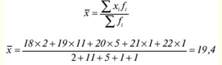 There is a certain rule for choosing a weighted arithmetic mean: if there is a series of data on two interrelated indicators, for one of which it is necessary to calculate the average value, and at the same time, the numerical values of the denominator of its logical formula are known, and the values of the numerator are not known, but can be found as a product of these indicators, then the average value should be calculated according to the formula of the arithmetic weighted average. In some cases, the nature of the initial statistical data is such that the calculation of the arithmetic mean loses its meaning and the only generalizing indicator can only be another type of average - the harmonic mean. At present, the computational properties of the arithmetic mean have lost their relevance in the calculation of generalizing statistical indicators due to the widespread introduction of electronic computers. The average harmonic value, which is also simple and weighted, has acquired great practical importance. If the numerical values of the numerator of the logical formula are known, but the values of the denominator are not known, then the average value is calculated by the weighted harmonic mean formula. If, when using the average harmonic weight of all options (f;) are equal, then instead of the weighted one, you can use a simple (unweighted) harmonic mean:  where x - individual options; n is the number of variants of the averaged feature. For example, a simple harmonic mean can be applied to speed if the segments of the path traveled at different speeds are equal. Any average value should be calculated so that when it replaces each variant of the averaged feature, the value of some final, generalizing indicator, which is associated with the averaged indicator, does not change. So, when replacing the actual speeds on individual sections of the path with their average value, the average speed) should not change the total distance. The average formula is determined by the nature (mechanism) of the relationship of this final indicator with the average. Therefore, the final indicator, the value of which should not change when the options are replaced by their average value, is called the defining indicator. To derive the average formula, you need to compose and solve an equation using the relationship of the averaged indicator with the determining one. This equation is constructed by replacing the variants of the averaged feature (indicator) with their average value. In addition to the arithmetic mean and the harmonic mean, other types (forms) of the mean are also used in statistics. All of them are special cases of the power mean. If you calculate all types of power-law averages for the same data, then their values will be the same, here the rule of majorance of averages applies. As the exponent of the mean increases, so does the mean itself. The geometric mean is used when there are n growth factors, while the individual values of the attribute are, as a rule, relative values of the dynamics, built in the form of chain values, as a ratio to the previous level of each level in the dynamics series. The average thus characterizes the average growth rate. The geometric simple mean is calculated by the formula:  The formula for the geometric weighted average is as follows:  The above formulas are identical, but one is applied at current coefficients or growth rates, and the second - at the absolute values of the levels of the series. The root mean square is used when calculating with the values of square functions, it is used to measure the degree of fluctuation of the individual values of a trait around the arithmetic mean in the distribution series and is calculated by the formula:  The weighted root mean square is calculated using a different formula:  The average cubic is used when calculating with the values of cubic functions and is calculated by the formula:  and the average cubic weighted:  All the above average values can be represented as a general formula:  where x is the average value; x - individual value; n is the number of units of the studied population; k - exponent that determines the type of average. When using the same initial data, the more k in the general power mean formula, the greater the average value. It follows from this that there is a regular relationship between the values of power means:  The average values described above give a generalized idea of the population under study, and from this point of view, their theoretical, applied, and cognitive significance is indisputable. But it happens that the value of the average does not coincide with any of the really existing options. Therefore, in addition to the considered averages, in statistical analysis it is advisable to use the values of specific options that occupy a well-defined position in an ordered (ranked) series of characteristic values. Among such quantities, the most common are structural (or descriptive) averages - mode (Mo) and median (Me). Fashion - the value of the trait that is most often found in this population. In relation to the variational series, the mode is the most frequently occurring value of the ranked series, i.e., the variant with the highest frequency. Fashion can be used to determine the most visited stores, the most common price for any product. It shows the size of the feature, characteristic of a significant part of the population, and is determined by the formula:  where x0 - the lower limit of the interval; h is the value of the interval; fm- interval frequency; fm1- frequency of the previous interval; fm + 1- frequency of the next interval. median the variant located in the center of the ranked row is called. The median divides the series into two equal parts in such a way that on both sides of it there is the same number of population units. At the same time, in one half of the population units, the value of the variable attribute is less than the median, in the other half it is greater than it. The median is used when examining an element whose value is greater than or equal to or simultaneously less than or equal to half of the elements of the distribution series. The median gives a general idea of where the values of the feature are concentrated, in other words, where is their center. The descriptive nature of the median is manifested in the fact that it characterizes the quantitative boundary of the values of the varying attribute, which are possessed by half of the population units. The problem of finding the median for a discrete variational series is solved simply. If all units of the series are given serial numbers, then the serial number of the median variant is defined as (n + 1) / 2 with an odd number of members n. If the number of members of the series is an even number, then the median will be the average of two variants with serial numbers n / 2 and n/2 + 1. When determining the median in interval variation series, the interval in which it is located (the median interval) is first determined. This interval is characterized by the fact that its accumulated sum of frequencies is equal to or exceeds half the sum of all frequencies of the series. The calculation of the median of the interval variation series is carried out according to the formula:  where x0 - the lower limit of the interval; h is the value of the interval; fm- interval frequency; f is the number of members of the series; ∫ m -1 - the sum of the accumulated members of the series preceding this one. Along with the median, for a more complete characterization of the structure of the studied population, other values of options are used, which occupy a quite definite position in the ranked series. These include quartiles and deciles. Quartiles divide the series by the sum of frequencies into four equal parts, and deciles - into ten equal parts. There are three quartiles and nine deciles. The median and mode, in contrast to the arithmetic mean, do not cancel out individual differences in the values of a variable attribute and, therefore, are additional and very important characteristics of a statistical population. In practice, they are often used instead of the average or along with it. It is especially expedient to calculate the median and mode in those cases when the studied population contains a certain number of units with a very large or very small value of the variable attribute. These values of options, which are not very characteristic for the population, while affecting the arithmetic mean, do not affect the values of the median and mode, which makes the latter very valuable indicators for economic and statistical analysis. 3. Indicators of variation The purpose of a statistical study is to identify the main properties and patterns of the studied statistical population. In the process of summary processing of statistical observation data, distribution series are built. There are two types of distribution series - attributive and variational - depending on whether the attribute taken as the basis of the grouping is qualitative or quantitative. Variation series are called distribution series built on a quantitative basis. The values of quantitative characteristics for individual units of the population are not constant, they differ more or less from each other. This difference in the size of a trait is called variation. Separate numerical values of a feature that occur in the studied population are called value variants. The presence of variation in individual units of the population is due to the influence of a large number of factors on the formation of the trait level. The study of the nature and degree of variation of signs in individual units of the population is the most important issue of any statistical study. Variation indicators are used to describe the measure of trait variability. Another important task of statistical research is to determine the role of individual factors or their groups in the variation of certain features of the population. To solve such a problem in statistics, special methods for studying variation are used, based on the use of a system of indicators that measure variation. In practice, the researcher is faced with a sufficiently large number of options for the values of the attribute, which does not give an idea of the distribution of units according to the value of the attribute in the aggregate. To do this, all variants of the attribute values are arranged in ascending or descending order. This process is called series ranking. The ranked series immediately gives a general idea of the values that the feature takes in the aggregate. The insufficiency of the average value for an exhaustive characterization of the population makes it necessary to supplement the average values with indicators that make it possible to assess the typicality of these averages by measuring the fluctuation (variation) of the trait under study. The use of these indicators of variation makes it possible to make the statistical analysis more complete and meaningful, and thus to better understand the essence of the studied social phenomena. The simplest signs of variation are minimum and maximum - this is the smallest and largest value of the feature in the aggregate. The number of repetitions of individual variants of feature values is called the frequency of repetition. Frequency - a relative indicator of frequency, which can be expressed in fractions of a unit or a percentage, allows you to compare variation series with a different number of observations. Formally we have:  where fi - number of options. To measure the variation of a trait, various absolute and relative indicators are used. The absolute indicators of variation include the mean linear deviation, the range of variation, variance, standard deviation. The range of variation (R) is the difference between the maximum and minimum values of the trait in the studied population, formally we have: R=XMax- Xmin This indicator gives only the most general idea of the fluctuation of the trait under study, because it shows the difference only between the limiting values of the options. It is completely unrelated to the frequencies in the variation series, i.e., to the nature of the distribution, and its dependence only on the extreme values of the attribute can give it an unstable, random character. The range of variation does not provide any information about the features of the studied populations and does not allow assessing the degree of typicality of the obtained averages. The scope of this indicator is limited to fairly homogeneous aggregates. More precisely, the indicator characterizes the variation of a trait, based on taking into account the variability of all values of the trait. To characterize the variation of a trait, one must be able to generalize the deviations of all these values from some typical value for the population under study. Variation indicators such as the mean linear deviation, variance and standard deviation are based on the consideration of deviations of the values of the attribute of individual population units from the arithmetic mean. Average linear deviation is the arithmetic mean of the absolute values of the deviations of individual options from their arithmetic mean:  where d is the average linear deviation; |x−x| - the absolute value (modulus) of the deviation of the variant from the arithmetic mean; f - frequency. The first formula is applied if each of the options occurs in the aggregate only once, and the second - in series with unequal frequencies. There is another way to average the deviations of options from the arithmetic mean. This method, which is very common in statistics, is reduced to calculating the squared deviations of options from the mean and then averaging them. In this case, we get a new indicator of variation - the variance. variance (σ2) - the average of the squared deviations of the variants of the trait values from their average value: 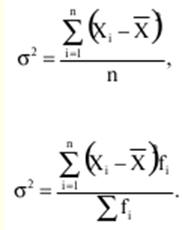 The second formula is used if the variants have their own weights (or frequencies of the variation series). In economic and statistical analysis, it is customary to evaluate the variation of an attribute most often using the standard deviation. Standard deviation (σ) is the square root of the variance:  The mean linear and mean square deviations show how much the value of the attribute fluctuates on average for the units of the population under study, and are expressed in the same units as the variants. In statistical practice, it often becomes necessary to compare the variation of various features. For example, it is of great interest to compare variations in the age of personnel and their qualifications, length of service and wages, etc. For such comparisons, indicators of the absolute variability of characteristics (average linear and standard deviation), of course, are unsuitable. It is impossible, in fact, to compare the fluctuation of work experience, expressed in years, with the fluctuation of wages, expressed in rubles and kopecks. When comparing the variability of various traits in the aggregate, it is convenient to use relative indicators of variation. These indicators are calculated as the ratio of absolute indicators to the arithmetic mean (or median). Using the range of variation, the average linear deviation, the standard deviation as an absolute indicator of variation, one obtains the relative indicators of fluctuation:  The coefficient of variation is the most commonly used indicator of relative volatility, characterizing the homogeneity of the population. The set is considered homogeneous if the coefficient of variation does not exceed 33% for distributions close to normal. LECTURE №6. Selective observation 1. General concept of selective observation Statistical observation can be organized as continuous and non-continuous. Continuous involves the examination of all units of the studied population of the phenomenon, non-continuous - only its parts. Selective observation also belongs to discontinuous. Selective observation is one of the most widely used types of non-continuous observation. This observation is based on the idea that some of the units selected in a random order can represent the entire studied set of the phenomenon according to the characteristics of interest to the researcher. The purpose of sample observation is to obtain information, first of all, to determine the summary generalizing characteristics of the entire population under study. In its purpose, selective observation coincides with one of the tasks of continuous observation, and therefore it can be a matter of which of the two types of observation - continuous or selective - is more appropriate to carry out. When resolving this issue, it is necessary to proceed from the following basic requirements for statistical observation: 1) information must be reliable, i.e., correspond to reality as much as possible; 2) the information must be complete enough to solve the research problems; 3) the selection of information should be carried out as soon as possible to ensure its use for operational purposes; 4) monetary and labor costs for organizing and conducting should be minimal. With selective observation, these requirements are met to a greater extent than with continuous observation. The advantages of selective observation in comparison with continuous observation can be fully appreciated if it is organized and carried out in strict accordance with the scientific principles of the theory of the sampling method. Such a principle is to ensure the randomness of the selection of units and their sufficient number. Compliance with the principle makes it possible to obtain such a set of units that, according to the features of interest to the researcher, represents the entire studied set, i.e., is representative (representative). When conducting selective observation, not all units of the object under study are examined, that is, not all units of the general population, but only some part of it, specially selected. The first principle of selection - ensuring randomness - is that when selecting each of the units of the population under study, an equal opportunity to get into the sample is provided. Random selection is not random selection. Random selection can only be ensured by following a certain methodology (for example, by selecting by lot, using tables of random numbers, etc.). The second principle of selection - ensuring a sufficient number of selected units - is closely related to the concept of representativeness of the sample. The concept of the representativeness of the selected set of units should not be understood as its representativeness in all respects, i.e., in all respects of the studied population. It is almost impossible to provide such representation. Any sample observation is carried out with a specific purpose and clearly formulated specific tasks, and the concept of representativeness should be associated with the purpose and objectives of the study. The part selected from the entire studied population should be representative, first of all, in relation to those features that are being studied or have a significant impact on the formation of summary generalizing characteristics. Let us introduce some concepts used in selective observation. General population the entire studied set of units is called, which is subject to study according to the characteristics of interest to the researcher. sampling set some part of it selected randomly from the general population is called. This sample is subject to the requirement of representativeness, which means the possibility, by studying only a part of the general population, to extend the findings to the entire population. The characteristics of the general and sample populations can be the average values of the studied features, their variances and standard deviations, mode and median, etc. Researchers may also be interested in the distribution of units according to the characteristics under study in the general and sample populations. In this case, the frequencies are called general and sample frequencies, respectively. The system of selection rules and ways of characterizing the units of the population under study constitutes the content of the sampling method. The essence of the sampling method is to obtain primary data, carried out by observing the sample, followed by generalization, analysis and distribution to the entire population in order to obtain reliable information about the phenomenon under study. The representativeness of the sample is ensured by the observance of the principle of random selection of objects in the population in the sample. If the population is qualitatively homogeneous, then the principle of randomness is implemented by a simple random selection of sample objects. Simple random selection is such a sampling procedure that provides the same probability for each unit of the population to be selected for observation, for any sample of a given size. So, the purpose of the sampling method is to draw a conclusion about the value of the characteristics of the general population based on information from a random sample from this population. 2. Sampling errors Between the characteristics of the sample population and the characteristics of the general population, as a rule, there is some discrepancy, which is called the error of statistical observation. During mass observation, errors are inevitable, but they arise as a result of various reasons. The value of a possible error of a sample attribute is made up of registration errors and representativeness errors. Registration errors, or technical errors, are associated with insufficient qualifications of observers, inaccurate calculations, imperfection of instruments, etc. Under representativeness (representation) error understand the discrepancy between the sample characteristic and the estimated characteristic of the general population. Representativeness errors can be random or systematic. Systematic errors are associated with violation of established selection rules. Random errors are explained by insufficiently uniform representation in the sample set of various categories of units of the general population. As a result of the first reason, the sample can easily turn out to be biased, since in the selection of each unit an error is made, always directed in the same direction. This error is called the offset error. Its size may exceed the value of a random error. A feature of the bias error is that, being a constant part of the representativeness error, it increases with the sample size. Random error decreases as the sample size increases. In addition, the magnitude of the random error can be determined, while the magnitude of the bias error is very difficult, and sometimes impossible, to directly determine in practice. Therefore, it is important to know the causes of the offset error and to provide measures to eliminate it. Bias errors are either intentional or unintentional. The reason for the intentional error is a biased approach to the selection of units from the general population. In order to prevent the occurrence of such an error, it is necessary to observe the principle of random selection of units. Unintentional errors can occur at the stage of preparing a sample observation, forming a sample population and analyzing its data. To avoid such errors, a good sampling frame is needed, i.e. the population from which it is intended to be selected, for example, a list of sampling units. The sampling frame must be reliable, complete and consistent with the purpose of the study, and the sampling units and their characteristics must correspond to their actual state at the time the sampling was prepared. It is not uncommon for some units in the sample to be difficult to collect information due to their absence at the time of observation, unwillingness to provide information, etc. In such cases, these units have to be replaced by others. It is necessary to ensure that the replacement is carried out by equivalent units. Random sampling error occurs as a result of random differences between the units in the sample and the units of the general population, i.e. it is associated with random selection. The theoretical justification for the appearance of random sampling errors is the theory of probability and its limit theorems. The essence of limit theorems is that in mass phenomena the cumulative influence of various random causes on the formation of regularities and generalizing characteristics will be an arbitrarily small value or practically does not depend on the case. Since random sampling error occurs as a result of random differences between the units of the sample and the general population, then with a sufficiently large sample size, it will be arbitrarily small. The limit theorems of probability theory allow one to determine the size of random sampling errors. Distinguish between the mean (standard) and marginal sampling errors. Under average (standard) error sampling refers to the discrepancy between the sample mean and the population mean. marginal error It is customary to consider the maximum possible discrepancy, i.e., the maximum error for a given probability of its occurrence, as a sample. In the mathematical theory of the sampling method, the average characteristics of the characteristics of the sample and the general population are compared and it is proved that with an increase in the sample size, the probability of large errors and the limits of the maximum possible error decrease. The more units are surveyed, the smaller the discrepancy between the sample and general characteristics will be. Based on the theorem proved by P. L. Chebyshev, the value of the standard error of a simple random sample with a sufficiently large sample size (n) can be determined by the formula:  where µxis standard error. From this formula for the mean (standard) error of a simple random sample, it can be seen that the value µx depends on the variability of the trait in the general population (the greater the variation of the trait, the greater the sampling error) and on the sample size n, the more units are surveyed, the smaller the discrepancy between the sample and general characteristics). Academician A. M. Lyapunov proved that the probability of occurrence of a random sampling error with a sufficiently large size of it obeys the law of normal distribution. This probability is determined by the formula:  In mathematical statistics, the confidence factor t is used, and the values of the function F(t) are tabulated at different values of it, and the corresponding levels of confidence are obtained. The confidence coefficient allows you to calculate the marginal sampling error, calculated by the formula:  It follows from the formula that the marginal sampling error is equal to - times the number of average sampling errors. Thus, the marginal sampling error value can be set with a certain probability. Sample observation makes it possible to determine the arithmetic mean of the sample x and the marginal error of this average Δx, which shows with a certain probability) how much the sample can differ from the general average up or down. Then the value of the general average will be represented by an interval estimate, for which the lower bound will be equal to  The interval in which the unknown value of the estimated parameter will be enclosed with a given degree of probability is called the confidence interval, and the probability P is called the confidence probability. Most often, the confidence probability is taken equal to 0,95 or 0,99, then the confidence coefficient t is equal to 1,96 and 2,58, respectively. This means that the confidence interval contains the general mean with a given probability. Along with the absolute value of the marginal sampling error, the relative sampling error is also calculated, which is defined as the percentage of the marginal sampling error to the corresponding characteristic of the sampling population:  The greater the value of the marginal sampling error, the greater the value of the confidence interval and, consequently, the lower the accuracy of the estimate. The average (standard) error of the sample depends on the sample size and the degree of variation of the trait in the general population. 3. Determining the required sample size One of the scientific principles in sampling theory is to ensure that a sufficient number of units are selected. Theoretically, the need to comply with this principle is presented in the proofs of the limit theorems of probability theory, which allow you to establish how many units should be selected from the general population so that it is sufficient and ensures the representativeness of the sample. A decrease in the standard error of the sample (and hence an increase in the accuracy of the estimate) is always associated with an increase in the sample size. Therefore, already at the stage of organizing a sample observation, it is necessary to decide what the size of the sample should be in order to ensure the required accuracy of the observation results. The calculation of the required sample size is built using formulas derived from the formulas for the marginal sampling errors (∆) corresponding to one or another type and method of selection. So, for a random repeated sample size (n), we have:   The meaning of this formula is that in the case of random re-selection of the required number, the sample size is directly proportional to the square of the confidence coefficient (t2) and the variance of the variation feature (σ2) and is inversely proportional to the square of the marginal sampling error (∆2). In particular, with a 2-fold increase in the marginal error, the required sample size can be reduced by a factor of 4. Of the three parameters, two (t and ∆) are set by the researcher. At the same time, the researcher, based on the purpose and objectives of the sample survey, must decide in what quantitative combination it is better to include these parameters in order to provide the best option. In one case, he may be more satisfied with the reliability of the obtained results (t) than with the measure of accuracy (∆), in the other - vice versa. It is more difficult to resolve the issue of the magnitude of the marginal sampling error, since the researcher does not have this indicator at the stage of designing a sample observation. Therefore, in practice it is customary to set the value of the marginal sampling error, as a rule, within the range of up to 10% of the expected average level of the feature. Establishing an assumed average level can be approached in different ways: using data from similar earlier surveys, or using data from the sampling frame and taking a small pilot sample. The question of determining the required sample size becomes more complicated if the sample survey involves the study of several features of sampling units. In this case, the average levels of each of the characteristics and their variation, as a rule, are different, and therefore it is possible to decide which dispersion of which of the characteristics to give preference to only taking into account the purpose and objectives of the survey. When designing a sample observation, a predetermined value of the permissible sampling error is assumed in accordance with the objectives of a particular study and the probability of conclusions based on the results of the observation. In general, the formula for the marginal error of the sample mean allows us to solve the following problems: 1) determine the magnitude of possible deviations of the indicators of the general population from the indicators of the sample population; 2) to determine the required sample size, providing the required accuracy, in which the limits of a possible error will not exceed a certain, predetermined value; 3) determine the probability that the error in the sample will have a given limit. 4. Methods of selection and types of sampling In the theory of the sampling method, various methods of selection and types of sampling have been developed to ensure representativeness. Under selection method understand the procedure for selecting units from the general population. There are two methods of selection: repeated and non-repeated. In re-sampling, each randomly selected unit after its survey is returned to the general population and, with subsequent selection, may again fall into the sample. This selection method is built according to the "returned ball" scheme. With this method of selection, the probability of getting into the sample for each unit of the general population does not change regardless of the number of selected units. With non-repetitive selection, each unit selected at random, after its examination, is not returned to the general population. This selection method is built according to the "unreturned ball" scheme. The probability of being selected for each unit of the population increases as selection is made. Depending on the sampling methodology, the following main types of sampling are distinguished: random, mechanical, typical (stratified, regionalized), serial (nested), combined, multi-stage, multi-phase, interpenetrating. The actual random sample is formed in strict accordance with the scientific principles and rules of random selection. To obtain a proper random sample, the population is strictly divided into sampling units, and then a sufficient number of units is selected in a random repeated or non-repetitive order. A random order is an order equivalent to a draw. In practice, this order is best ensured by using special tables of random numbers. If, for example, 1587 units should be selected from a population containing 40 units, then 40 four-digit numbers that are less than 1587 are selected from the table. With a non-repetitive selection method, the calculation of the standard error is carried out using the formula: 
Since this proportion is always less than one, the error in non-repetitive selection, other things being equal, is always less than in repeated selection. Non-repetitive selection is practically always easier to organize than repeated selection, and it is used more often. Forming a sample in strict accordance with the rules of random selection is practically very difficult, and sometimes impossible, since when using tables of random numbers, it is necessary to number all units of the general population. Quite often, the population is so large that it is extremely difficult and impractical to carry out such preliminary work. Therefore, in practice, other types of samples are used, each of which is not strictly random. However, they are organized in such a way that the maximum approximation to the conditions of random selection is ensured. With a purely mechanical sample, the entire population of units must first of all be presented in the form of a list of units of selection, compiled in some neutral order with respect to the trait under study, for example, alphabetically. Then the list of sampling units is divided into as many equal parts as it is necessary to select units. Further, according to a predetermined rule, not related to the variation of the trait under study, one unit is selected from each part of the list. This type of sampling may not always provide a random selection, and the resulting sample may be biased. This is explained by the fact that, firstly, the ordering of the units of the general population can have an element of a non-random nature. Second, sampling from each part of the population, if the origin is incorrectly established, can also lead to a bias error. However, it is practically easier to organize a mechanical sample than a proper random one, and this type of sampling is most often used in sample surveys. Typical (zoned, stratified) sampling has two goals: 1) to ensure the representation in the sample of the corresponding typical groups of the general population according to the characteristics of interest to the researcher; 2) increase the accuracy of the sample survey results. With a typical sample, before the start of its formation, the general population of units is divided into typical groups. In this case, a very important point is the correct choice of a grouping attribute. Selected typical groups may contain the same or different number of selection units. In the first case, the sampling set is formed with the same share of selection from each group, in the second - with a share proportional to its share in the general population. If the sample is formed with an equal share of selection, in essence, it is equivalent to a number of proper random samples from smaller populations, each of which is a typical group. The selection from each group is carried out in a random (repeated or non-repeated) or mechanical order. With a typical sample (both with an equal and unequal selection share), it is possible to eliminate the influence of intergroup variation of the studied trait on the accuracy of its results, since the mandatory representation of each of the typical groups in the sample population is ensured. The standard error of the sample will not depend on the value of the total variance - σ2, and on the value of the average of the group dispersions σi2. Since the mean of the group variances is always less than the total variance, then, other things being equal, the standard error of a typical sample will be less than the standard error of a random sample itself. When determining the standard errors of a typical sample, the following formulas are used: 1) with the repeated selection method:  2) with a non-repetitive selection method:  where σв2- the average of the group variances in the sample population. Serial (nested) sampling - this is a type of sample formation, when not the units to be surveyed, but groups of units (series, nests) are randomly selected. Within the selected series (nests), all units are examined. Serial sampling is practically easier to organize and conduct than the selection of individual units. However, with this type of sampling, firstly, the representation of each of the series is not ensured, and, secondly, the influence of the interseries variation of the studied trait on the survey results is not eliminated. When this variation is significant, it will increase the random representativeness error. When choosing the type of sample, the researcher must take this circumstance into account. The standard error of serial sampling is determined by the formulas: 1) with the repeated selection method:  where σв2- interseries variance of the sample population; r - number of selected series; 2) with a non-repetitive selection method:  where R is the number of series in the general population. In practice, certain methods and types of sampling are used depending on the purpose and objectives of sample surveys, as well as the possibilities of organizing and conducting them. Most often, a combination of sampling methods and types of sampling is used. Such samples are called combined. Combination is possible in different combinations: mechanical and serial sampling, typical and mechanical, serial and random, etc. Combined sampling is used in order to ensure the greatest representativeness with the lowest labor and monetary costs for organizing and conducting the survey. With a combined sample, the value of the standard error of the sample consists of the errors at each of its steps and can be determined as the square root of the sum of the squares of the errors of the corresponding samples. So, if mechanical and typical sampling were used in combination with combined sampling, then the standard error can be determined by the formula:  where μ1 and μ2are the standard errors of the mechanical and typical samples, respectively. A feature of a multi-stage sample is that the sample is formed gradually, according to the selection steps. At the first stage, units of the first stage are selected using a predetermined method and type of selection. At the second stage, from each unit of the first stage included in the sample, units of the second stage are selected, and so on. The number of stages may be more than two. At the last stage, a sample is formed, the units of which are subject to survey. So, for example, for a sample survey of household budgets, at the first stage, territorial subjects of the country are selected, at the second stage, districts in the selected regions, at the third stage, enterprises or organizations are selected in each municipality, and, finally, at the fourth stage, families are selected in the selected enterprises. Thus, the sampling set is formed at the last stage. Multi-stage sampling is more flexible than other types, although in general it gives less accurate results than a single-stage sample of the same size. However, at the same time, it has one important advantage, which is that the sampling frame in multi-stage selection needs to be built at each stage only for those units that are in the sample, and this is very important, since there is often no ready-made sampling frame. The standard error of sampling in multi-stage selection with groups of different volumes is determined by the formula:  where μ1, m2, m3,… - standard errors at different stages; n1, N2, N3,… - the number of samples at the corresponding stages of selection. In the event that the groups are not the same in size, theoretically this formula cannot be used. But if the total proportion of selection at all stages is constant, then in practice the calculation by this formula will not lead to a distortion of the error. The essence of a polyphase sample is that, based on the initially formed sample, a subsample is formed, from this subsample, the next subsample, etc. The initial sample is the first phase, the subsample from it is the second, etc. Polyphase sample useful in several cases: 1) if an unequal sample size is required to study various features; 2) if the fluctuation of the studied features is not the same and the required accuracy is different; 3) if in relation to all units of the initial sample (first phase) it is necessary to collect one - less detailed information, and in relation to the units of each subsequent phase - others - more detailed. One of the undoubted advantages of a multi-phase sample is the fact that the information obtained in the first phase can be used as additional information in subsequent phases, the information of the second phase can be used as additional information in the following phases, etc. This use of information increases the accuracy of the results of a sample survey. . When organizing a multi-phase sampling, a combination of various methods and types of selection can be used (typical sampling with mechanical sampling, etc.). Multi-phase selection can be combined with multi-stage. At each stage, the sampling can be multi-phase. The standard error in a multi-phase sample is calculated for each phase separately in accordance with the formulas of the selection method and type of sample, with the help of which its sample was formed. Interpenetrating samples are two or more independent samples from the same general population, formed by the same method and type. It is advisable to resort to interpenetrating samples if it is necessary to obtain preliminary results of sample surveys in a short time. Interpenetrating samples are effective for evaluating survey results. If the results are the same in independent samples, then this indicates the reliability of the sample survey data. Interpenetrating samples can sometimes be used to test the work of different researchers by having each researcher conduct a different sample survey. The standard error for interpenetrating samples is defined in the same way as for typical proportional sampling. Interpenetrating samples require more labor and money than other types, so the researcher must take this into account when designing a sample survey. Limit errors for various selection methods and types of sampling are determined by the formula: Δ = tμ, where μ is the corresponding standard error. LECTURE №7. Index Analysis 1. General concept of indices and index method In the practice of statistics, indices, along with averages, are the most common statistical indicators. With their help, the development of the national economy as a whole and its individual sectors is characterized, the role of individual factors in the formation of the most important economic indicators is studied. Indices are also used in international comparisons of economic indicators, determining the standard of living, monitoring business activity in the economy, etc. Index (lat. Index) is a relative value showing how many times the level of the studied phenomenon under given conditions differs from the level of the same phenomenon in other conditions. The difference in conditions can manifest itself in time (indices of dynamics), in space (territorial indices) and in the choice of some conditional level as the basis for comparison. According to the coverage of the elements of the population (its objects, units and their characteristics), individual (elementary) and summary (complex) indices are distinguished, which are divided into general and group. Individual indices - this is the result of comparing two indicators related to the same object, for example, comparing the prices of a product, the volume of its sale, etc. In the statistical and economic analysis of the activities of enterprises and industries, individual indices of qualitative and quantitative indicators are widely used, for example, the price index . Determined by the formula:  The price index characterizes the relative change in the unit price level of each type of product in the reporting period compared to the baseline and is a qualitative indicator. The physical volume index is determined by the formula:  The physical volume index shows how many times the production of this type of product has changed in the reporting period in relation to the period with which the comparison was made, and is a quantitative indicator. The composite index characterizes the ratio of the levels of several elements of the population (for example, a change in the volume of output of several types of products that have a different natural-material form, or a change in the level of labor productivity in the production of several types of products). If the population under study consists of several groups, then the composite indices, each of which characterizes the change in the levels of a separate group of units, are group (sub-indices), and the composite index, covering the entire population of units, is a general (total) index. Composite indices express the ratio of complex socio-economic phenomena and consist of two parts: 1) from the indexed value; 2) from a co-meter, which is called weight. The indicator, the change of which characterizes the index, is called indexed. Indexed indicators can be of two kinds. Some of them measure the general, total size (volume) of a particular phenomenon and are conditionally called volumetric, extensive (quantity, i.e., the physical volume of a given type of product, the number of employees, the total labor costs for production, the total cost of production, etc.). P.). These indicators are obtained as a result of direct calculation or summation and are initial, primary. Other indicators measure the level of a phenomenon or feature in terms of one or another unit of the population and are conditionally called qualitative, intensive: production output per unit of time (or per employee), working time per unit of production, unit cost of production, etc. These indicators are obtained by dividing volumetric indicators, i.e., they are of a calculated, secondary nature. They measure the intensity, effectiveness of a phenomenon or process and, as a rule, are either average or relative values. When using the index method, a certain symbolism is applied, i.e., a system of conventions. Each indexed indicator is denoted by a specific letter, usually Latin): Q - the quantity (volume) of manufactured products (or the quantity of goods sold) of this type in physical terms; T - the total cost of working time (labor) for the production of this type of product, measured in man-hours or man-days; in some cases, the same letter indicates the average payroll number of employees; z - unit cost of production; p is the price of a unit of production or goods; M - the total consumption of raw materials, material or fuel for the production of products of a given type and volume. Indicators for the base period have a subscript "0" in the formulas, and for the compared (current, reporting) period - the sign "1". Individual indices are denoted by the letter i and are also provided with a subscript - the designation of the indexed indicator. Yes, 1Q means an individual index of the quantity (physical volume) of manufactured products (or goods sold) of a given type; iz - individual unit cost index of a given type of product, etc. Composite indices are denoted by the letter I and are also accompanied by subscript indicators of the indicators whose change they characterize. For example, It - composite index of labor intensity of a unit of production, etc. Individual indices are ordinary relative values, that is, they can be called indices only in the broad sense of this term. Indices in the narrow sense, or indices proper, are also relative indicators, but of a special kind. They have a more complex method of construction and calculation, and the specific methods of their construction are the essence of the index method. Socio-economic phenomena and indicators characterizing them can be commensurate, that is, have a common measure, and incommensurable. Thus, the volumes of products or goods of the same type and variety produced at different enterprises or sold in different stores are commensurate and can be summed up, while the volumes of different types of products or goods are incommensurable and cannot be directly summed up. It is impossible, for example, to add kilograms of bread with liters of milk, meters of cloth and pairs of shoes. The incommensurability and impossibility of direct summation in the construction and calculation of the composite index are explained here not so much by the difference in natural units of measurement as by the difference in consumer properties, the unequal natural-material form of these products or goods. In this regard, in order to calculate composite indices, it is necessary to bring their constituent parts to a comparable form. The unity of different types of products or different goods lies in the fact that they are products of labor, have a certain value and its monetary expression - the price (p). Each product also has a particular cost (z) and labor intensity (t). These qualitative indicators can be used as a general measure - the coefficients of comparison of heterogeneous products. By multiplying the volume of each kind of product (Q) by the corresponding price, cost or labor intensity of a unit of production, we will reduce the various products to the same unity and obtain comparable figures that can be summarized. The situation is similar when constructing composite indexes of qualitative indicators. Suppose, for example, we are interested in the change in the general price level of the various goods sold. Although formally the prices of different commodities are commensurable, their direct summation (without taking into account the quantity of each commodity sold) gives a value devoid of independent practical significance. Therefore, the composite price index cannot be constructed as a ratio of simple sums:  The prices of individual goods do not take into account the specific number of goods sold and their statistical weight and role in the process of commodity circulation. Simple sums of prices of individual goods are not suitable for building a composite index, also because prices depend on the unit of measurement of goods, the change of which will give different amounts and a different value of the index. Consequently, when constructing composite indices of qualitative indicators, they cannot be considered in isolation from the volumetric indicators associated with them, per unit of which these qualitative indicators are calculated. Only by multiplying one or another qualitative indicator (p, z, t) by a volume indicator (Q) directly related to them, it is possible to take into account the role and statistical weight of each type of product (or product) in a particular economic process - the process of formation of the total value ( pQ), the total cost (zQ), the total cost of working time (tQ), etc. At the same time, it is possible to obtain indicators whose summation is of practical importance. Thus, the first feature of the index method and the indices themselves is that the indexed indicator is not considered in isolation, but in conjunction with other indicators. By multiplying the indexed indicator by another, related to it, we reduce various phenomena to their unity, ensure their quantitative comparability and take into account their weight in the real economic process. Therefore, multiplier indicators associated with indexed indicators are usually called weights of indices, and multiplication by them is called weighting. However, multiplying the values of an indexed indicator by the values of another indicator (weight) associated with them does not yet solve the problem of the index itself. By multiplying, for example, the prices of the corresponding quantities of commodities, one can find the value of these commodities in each period, and thus the problem of commensuration and weighting can be solved. However, comparing the obtained sums of products (∑p1Q1 and ∑poQo) gives an indicator that characterizes the change in trade turnover, depending on two factors - prices and quantities (volumes) of goods, but does not characterize changes in the price level and the level of production of goods:  In order for the index to characterize the change in only one factor, it is necessary to eliminate the change in the other factor in the above formula, fixing it both in the numerator and in the denominator at the level of the same period. For example, to estimate the volume of heterogeneous products in two compared periods, it is necessary to evaluate the goods sold in both periods at the same, for example, basic, prices (p0). The resulting indicator will reflect the change in only one factor - the physical volume of production Q:  And to assess the change in the price level for a group of goods, it is necessary to compare the same volumes of these goods, i.e., the number of goods (Q) should be fixed both in the numerator and in the denominator of the index at the same level (either at the base or at the reporting level). Thus, the constructed composite price indices will characterize only the change in prices, i.e., the indexed indicator, since the change in weights (Q) will be eliminated (eliminated) due to their fixation:  In both cases (Tq and Tp) the index reflected the change in only one factor - the indexed indicator - due to the fixation of the other (weights) at the same level. Eliminating the influence of changing weights by fixing them in the numerator and denominator of the index at the same level is the second feature of indices and the index method. Considering the problems that arise in the construction of the actual indices, the task was to give a comparative description of the levels of a complex phenomenon consisting of heterogeneous elements (different types of products, etc.). Yes, Tp should show how the price level has changed in general, i.e., measure the price dynamics of various goods in the form of one generalizing indicator. Historically, the indices themselves appeared as a result of solving this particular economic task - the task of generalizing, synthesizing the dynamics of individual elements of a complex phenomenon in one generalizing indicator - a composite index. However, the indices themselves are used to solve another problem - to analyze the impact of changes in individual indicators-factors on the change in an indicator representing a function of these factors-arguments. Thus, the total cost of goods sold is a function of their prices (p) and quantities (volumes - Q). Therefore, it is possible to set the task to measure the influence of each of these factors on the change in turnover: to determine how it has changed separately due to changes in each factor. Indices used to solve such analytical problems are also built using the specific features of the index method - weighting and eliminating changes in weights. Thus, the index itself is a relative indicator of a special kind, in which the levels of a socio-economic phenomenon are considered in connection with another (or other) phenomenon, the change of which is eliminated in this case. Indicators associated with the indexed indicator are used as index weights, and weighting and elimination of weight changes (fixing in the numerator and denominator of the index at the same level) are the specifics of the indices themselves and the index method. 2. Aggregate indices of qualitative indicators Each qualitative indicator is associated with one or another volume indicator, based on the unit of measurement of which it is calculated (or to the unit of measurement of which it refers). Thus, the unit price of a good is related to its quantity (Q); quality indicators such as price (p), cost (z) and labor intensity are associated with the volume of production  units of production, as well as the specific consumption of raw materials, materials  Composite indices of quality indicators should not characterize their change in general in relation to any arbitrary set of goods or products, but the change in prices, prime cost, labor intensity or unit costs of a completely certain amount of goods produced or goods sold. This is achieved by weighting - multiplying the levels of the indexed qualitative indicator by the value of the volume indicator (weight) associated with it - and fixing the weights in the numerator and denominator of the index at the same level. Comparison of the sums of such products gives an aggregate index. Similarly, aggregate indices of the dynamics of the cost and labor intensity of a unit of production, as well as the index of the specific consumption of raw materials or materials, can be constructed. The main problem in constructing these composite indices is the economically justified choice of the level at which the weights of the index should be fixed, i.e., in this case, the volume of production (or goods) - Q. Usually, before the composite index of the dynamics of a qualitative indicator, the task is to measure not only the relative change in the level, but also the absolute value of the economic effect that is obtained in the current period as a result of this change: the amount of savings for buyers due to price reductions (or the amount of their additional costs, if prices increased), the amount of savings (or additional costs) due to changes in cost, etc. This formulation of the problem leads to indices of the dynamics of qualitative indicators with weights of the current period. First, the researcher is interested in the change in the cost or labor intensity of the products that are currently produced, and not in the past; secondly, the economic effect should be linked to the actual results of the current, reporting, and not the previous (base) period. Let's take the aggregate cost index as an example:  Thus, in this index, the numerator is the sum of actual costs for products in the reporting period, and the denominator is a conditional value that shows how much money would be spent on products in the reporting period if the unit cost of each type of product remained at the base level. The real economic effect obtained by changing the unit cost of production is expressed as an absolute value, which is calculated as the difference between the amounts in the numerator and denominator of the index   Therefore, weighting by the weights of the reporting (current) period links the index of the qualitative indicator with the indicator of the economic effect, which is obtained by changing the indexed indicator. Therefore, aggregate indices of the dynamics of qualitative indicators are usually built and calculated with the weights of the reporting period: 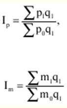 In these indices, the difference between the numerator and denominator characterizes: in the first case, a decrease or increase in the cost of acquiring the same set of goods, depending on the sign of the difference; in the second case - an increase or decrease in the consumption of materials for the production of the same volume of products. 3. Aggregate indices of volume indicators Volumetric indicators can be commensurate (the volume of products or goods of the same type) and incommensurable (the volume of products or goods of different types - Q). Comparable volume indicators can be directly summed up, and the construction of aggregate indices does not cause difficulties. To obtain a general result and build an aggregate index of a disparate volume indicator, it is necessary to first measure the individual values of this indicator. Based on the economic essence of the phenomenon, it is necessary to find a common measure and use it as a measurement coefficient. Such a common measure for volumetric indicators is the associated quality indicators with them. Thus, the volumes of various types of products can be measured using the price (p), cost (z) and labor intensity (t) of a unit of these products. By multiplying the indexed volume indicator by one or another qualitative indicator, one not only provides the possibility of summation, but at the same time also takes into account the role of each element, for example, a product, in the real economic process, i.e., its statistical weight in this process. Since various qualitative indicators can act as weights in the volume index, the question arises as to which of them should be used. This issue in each specific case must be resolved in accordance with the cognitive economic task that is put before the index, i.e., the choice of certain weights-commensurators must be economically justified. In the practice of economic and statistical work, prices are usually used as weights for the aggregate index of output. This is how indices of the volume of industrial and agricultural products are built, as well as indices of the physical volume of trade. In a number of cases, a change in the volume of production is of interest to us not in itself, but from the point of view of its influence on a change in an indicator of a more complex order - the total cost of production, its total cost, the total cost of working time, the total volume of production in a given section of it, etc. In such cases, the choice of weights-components is determined by the relationship of indicators-factors on which a more complex indicator depends. In order for the index to reflect only the change in the indexed volume indicator, the weights in its numerator and denominator are fixed at the level of the same period. In the practice of economic work in the indices of the dynamics of volume indicators, the weights are usually fixed at the level of the base period. This makes it possible to build systems of interconnected indexes. For individual volume indicators (sales volume, productivity volume, sown area), the weights are selected at the level of the base period. For example:  where In - composite yield index; Ip - composite index of the cost of goods turnover; Iq - consolidated cost index. Unlike quality indexes, which are calculated on a comparable range of units (comparable products), composite volume indexes, for the sake of completeness and accuracy, should cover the entire range of units produced or sold) in each period. In this regard, the question arises of what weights should be taken for those types of products that were not produced in one of the compared periods. In the practice of statistics in such cases, two methods are used. When calculating indices of the volume of industrial output, new types of industrial output for which there are no prices of the base period are estimated conditionally at the prices of the current period. When calculating the indices of the volume of goods sold, a method is used based on the conditional assumption that the prices of new goods have changed to the same extent as the prices of the comparable range of similar goods. 4. Series of aggregate indices with constant and variable weights When studying the dynamics of economic phenomena, indices are built and calculated for a number of successive periods. They form a series of either basic or chain indices. In a number of basic indices, the indexed indicator in each index is compared with the level of the same period, and in a number of chain indices, the indexed indicator is compared with the level of the previous period. In each individual index, the weights in its numerator and denominator are necessarily fixed at the same level. If a series of indices is being built, then the weights in it can be either constant for all indices of the series, or variable. A number of basic indices of production volume:  Constant weights (p0) also has a number of chain indices:  A number of chain price indices:  For dynamics indices with constant weights, the relationship between chain and basic growth rates (indices) is valid:  Thus, the use of constant weights over a number of years makes it possible to move from chain indices to basic ones, and vice versa. Therefore, the series of indices for the volume of production and the volume of goods sold are constructed in statistical practice with constant weights. For example, in volume indices, prices fixed at the level that was set on January 1 of any base year are used as constant weights. Such prices, used for a number of years, are called comparable (fixed). The use of comparable prices in the indices of the volume of production (goods) makes it possible, by simple summation, to obtain results for several years. Comparable prices should not differ significantly from current (current) prices. Therefore, they are periodically reviewed, moving to new comparable prices. In order to be able to calculate production volume indices for long periods during which different comparable prices were applied, the production of one year is valued both at the old and at the new fixed prices. The index for a long period is calculated by the chain method, that is, by multiplying the indices for individual segments of this period. The series of indexes of qualitative indicators, which are economically correct to weigh according to the weights of the current period, are constructed with variable weights. 5. Construction of consolidated territorial indices When constructing territorial indices, i.e., when comparing indicators in space (inter-district, comparison between different enterprises, etc.), questions arise about the choice of a comparison base and a region (object) at the level of which the index weights should be fixed. In each specific case, these issues need to be addressed based on the objectives of the study. The choice of the comparison base depends, in particular, on whether the comparisons will be bilateral (for example, comparing the indicators of two neighboring territorial units) or multilateral (comparing the indicators of several territories, objects). In two-sided comparisons, each territory or object with the same basis can be taken both as a comparison and as a comparison base. In this regard, the question arises of fixing the weights of the composite index at the level of a particular region (object). Let, for example, it is necessary to determine in which of the two areas and by how many percent the unit cost of production is lower and the volume of its production is greater. If we compare area A with area B, a fairly reasonable and simple way is to fix in the cost index as weights the volumes of production in general for both territories (Q = QA + QE), then you get:  With multilateral comparisons, for example, when comparing qualitative indicators in several areas, it is necessary to expand the boundaries of the territory at the level of which the weights are fixed accordingly. In the consolidated territorial indices of volume indicators, the average levels of the corresponding qualitative indicators, calculated as a whole for the compared territories, can be taken as weights. 6. Average indices Depending on the methodology for calculating individual and composite indices, there are arithmetic mean and mean harmonic indices. In other words, the overall index, built on the basis of the individual index, takes the form of an arithmetic average or harmonic index, i.e. it can be converted to an arithmetic average and a harmonic average. The idea of constructing a composite index as an average of individual (group) indices is quite natural, because the composite index is a general measure that characterizes the average change in the indexed indicator, and, of course, its value should depend on the values of individual indices. And the criterion for the correctness of constructing a composite index in the form of an average value (average index) is its identity to the aggregate index. The transformation of the aggregate index into the average of the individual (group) indices is carried out as follows: either in the numerator or in the denominator of the aggregate index, the indexed indicator is replaced by its expression in terms of the corresponding individual index. If such a replacement is made in the numerator, then the aggregate index will be converted into the arithmetic mean, if in the denominator, then into the harmonic mean of the individual indices. For example, the individual index of physical volume and the cost of production of each type in the base period are known (q0p0). The initial base for constructing the average of individual indices is the composite index of physical volume:  From the available data, only the denominator of the formula can be obtained directly by summation. The numerator can be obtained by multiplying the cost of an individual type of product of the base period by an individual index:  Then the formula of the composite index will take the form:  Consequently, we obtain the arithmetic average index of physical volume, where the weights are the cost of certain types of products in the base period. Let us assume that we have information about the dynamics of the volume of output of each type of product (iq) and the cost of each type of product in the reporting period (p1q1). To determine the overall change in the output of an enterprise in this case, it is convenient to use the Paasche formula:  The numerator of the formula can be obtained by summing the quantities q1p1, and the denominator - by dividing the actual cost of each type of product by the corresponding individual index of the physical volume of production, i.e. dividing p1q1 /iq, then:  Thus, we obtain the formula for the average weighted harmonic index of physical volume. The use of one or another formula for the index of physical volume (aggregate, arithmetic mean and harmonic mean) depends on the information available. You also need to keep in mind that the aggregate index can be converted and calculated as an average of individual indices only if the list of types of products or goods (their range) in the reporting and base periods coincides, i.e. when the aggregate index is built on a comparable range of units ( aggregate indices of qualitative indicators and aggregate indices of volume indicators, subject to a comparable assortment). LECTURE №8. Characteristics of the system of indicators that determine the economic activity of the enterprise 1. Principles for the formation of a system of indicators The general principle underlying the formation of a system of indicators of enterprise statistics is as follows. 1. The subject of statistics - this is the collection and processing of economic indicators that allow the analysis of the economic activity of enterprises of various types and industries. The collection of statistical information on the orders of specific consumers is carried out within the framework of industry statistics. For example, this is the activity of small enterprises. All information is divided into two streams: 1) the main results of all economic activities of small enterprises, regardless of their industry affiliation (form No. MP - T section, the most important economic indicators); 2) statistical indicators of the production of products or the provision of services in small enterprises of certain industries, including production in physical terms, are developed using the TT section of form No. MP and a number of industry forms, which are characterized by significant differentiation and detailing of the amount of information requested. Work is also underway to prepare baseline indicators for statistics on large and medium-sized enterprises. The areas of analysis of the activities of large and medium-sized enterprises, which determine the composition of the information collected in the framework of enterprise statistics, are: 1) the efficiency of the economic activity of the enterprise, the ratio of results and costs (the structure of profits and costs, profitability of production, the ratio of assets and liabilities, etc.); 2) financial and property status of enterprises (fixed and working capital, sources and directions of spending money, debt, etc.); 3) investment and business activity of enterprises (investments, production capacities and their use, the state of stocks, demand for products, labor movement, etc.); 4) structural and demographic characteristics of enterprises. Stages of work to determine the composition of the main economic indicators: 1) inventory and analysis of the current industry reporting in terms of the composition of indicators, the methodology for their formation, the timing of submission, the range of reporting units, etc.; 2) the formation of the main economic indicators of the micro level, taking into account the general structure of the conceptual scheme for analyzing the socio-economic development of Russia and the composition of individual special blocks; 3) comparison of the list of indicators with the statistical indicators available in the current reporting; 4) development of statistical reporting forms for large and medium enterprises; 5) preparation of proposals for the revision of the forms of statistical industry reporting. Industry reporting is valid in terms of production. It covers the issues of accounting for products in value and physical terms with all its calculations and reflects the specifics of the work of enterprises in a particular industry. Integrated reporting forms help eliminate the repeatability of statistical indicators, reduce the information burden on the enterprise. 2. Form of structural survey of enterprises is one example of integrated reporting forms for different types of manufacturers. The main to structural survey is the regular provision of statistical data on the state of the structure of the production system for a comprehensive analysis of the main parameters of the financial and economic activities of enterprises, the formation of individual macroeconomic indicators. 2. Manufacturing process. Characteristics of his model Manufacturing process is a set of separate labor processes aimed at the transformation of raw materials and materials into finished products. The composition of the production process has a certain impact on the construction of the enterprise and its production units. The production process is the basis of the economic activity of any enterprise. The main factors that help determine the nature of production are: 1) means of labor (machines, equipment, buildings, structures, etc.); 2) objects of labor (raw materials, materials, semi-finished products); 3) labor is the activity of people. The interaction of these main factors forms the composition of the production process. To labor resources refers to personnel, labor force, which is defined as a person's ability to work. Labor power in the production process is consumed in the form of living labor costs, measured by working time, as a natural measure of the purposeful activity of workers. An entrepreneur who uses personnel in his economic activity is faced with the fact that the labor force in the labor market is a particularly specific product that has a value. The amount of labor expended is expressed in monetary terms (wages). For an efficient production process, an entrepreneur must obtain sufficiently accurate and versatile information about the total amount of available labor resources, its qualitative characteristics (professional composition, qualifications, etc.) and the specifics of the formation of labor costs. Resources of means of labor is a set of various fixed production assets. The information subsystem of resources of labor means should contain indicators reflecting their availability, composition by type, technical condition and role in the formation of production and distribution costs. A feature of the means of labor is their functioning during several production cycles. The means of labor transfer their value to the product in parts, that is, as they wear out. In the production costs of one production cycle, the means of labor are included in the corresponding share of their depreciation, which is determined in monetary terms by the corresponding amount of depreciation. To the objects of work of the enterprise include: stocks of raw materials, materials, fuel and other material resources, including semi-finished products, components and stocks of goods. All these resources of the objects of labor of the enterprise are necessary for the normal course of production processes. In monetary terms, they form the bulk of the company's working capital, which also includes funds in settlements, free cash and other types of financial assets. To characterize the presence and use of objects of labor, the system of indicators should include data on their natural and material composition, availability, receipt and expenditure in the production process, characteristics of the efficiency of their consumption, etc., indicators that will determine the contribution of objects of labor to the formation of the total cost of the enterprise. The costs of production associated with the use of factors of production are transferred both to the total cost and to the cost of the product produced, which must exceed the total cost. The final result of the production process and circulation for the entrepreneur is clarified at the time of receipt of funds (revenue) received from buyers of the company's products in cash or non-cash form. The cash proceeds received by the entrepreneur are distributed in several directions, these are: 1) reimbursement of costs associated with the resumption of production in any amount determined by the owner of the company, which requires the investment of financial resources in the renewal of stocks of objects of labor to maintain and renew the resources of labor tools and to pay for the costs associated with the current consumption of living labor resources; 2) a part of the enterprise's proceeds is used by the entrepreneur to meet personal needs; 3) part of the proceeds goes to the environment external to the enterprise (payment of taxes, payments to off-budget and special funds, etc.). 3. Characteristics of systems of indicators that determine the resource potential and the results of all activities of the enterprise The role of labor resources is constantly increasing, and not only in the period of market relations. Labor collective - one of the main tasks of the entrepreneur, which is the key to the success of entrepreneurial activity, expression and prosperity of the entrepreneur. A team of like-minded people and partners who are able to realize, understand and implement the plans of the company's management is called a labor collective. Labor relations are a complex aspect of the enterprise. The production process depends on people, i.e. on their desire and ability to work and, accordingly, on their qualifications. The emerging new production systems do not only consist of machines, but also include people who work in close cooperation. Human capital, equipment and inventories are the cornerstone of competitiveness, economic growth and efficiency. The main factors influencing the increase in the efficiency of the enterprise: 1) selection and promotion of personnel; 2) training of personnel and their continuous education; 3) stability and flexibility of the composition of employees; 4) improvement of the material and moral evaluation of the work of employees. There are two criteria for selecting and promoting employees: 1) high professional qualification and ability to learn; 2) communication experience and willingness to cooperate. Employment security, reduced staff turnover, high wages provide a significant economic effect and create a desire among employees to improve work efficiency. Remuneration should stimulate the increase in labor productivity and have a motivational effect. To increase efficiency and productivity, it is necessary to change both wages and the approach to its formation. The organization of labor and management of the enterprise team includes: 1) hiring employees on a part-time or weekly basis; 2) the placement of workers in accordance with the established system of production; 3) distribution of duties among the employees of the enterprise; 4) retraining or training of personnel; 5) stimulation of labor; 6) improvement of labor organization. The labor collective of the enterprise adapts to the existing system of production processes. The structure of the production process is based on the scientific principles of labor organization, which include: 1) division of labor and improvement of its cooperation based on the division of the production process; 2) selection of professional and skilled workers and their placement; 3) improvement of labor processes through the development and implementation of rational labor methods and techniques; 4) improving the service of workplaces on the basis of a clear regulation of each service function; 5) the introduction of effective forms of teamwork, the development of multi-unit services and the combination of professions; 6) improvement of labor rationing based on the use of reserves, reducing labor costs and the most rational operating modes of equipment; 7) organization and conduct of systematic production briefing - advanced training of workers, exchange of experience and dissemination of advanced labor methods; 8) creation of sanitary and hygienic, psychophysiological, aesthetic conditions of work and work safety, the introduction of rational work schedules, work and rest regimes at work. General indicators of the implementation of these principles are: 1) growth of labor productivity; 2) satisfaction of all working conditions; 3) satisfaction with the content of labor and its attractiveness. The main sources of recruitment at the enterprise are all types of educational institutions, enterprises with similar professions, and the labor exchange. The distribution of duties and the placement of workers is based on a system of division of labor. The following forms of division of labor have become widespread: 1) technological - by types of work, professions and specialties; 2) operational - for certain types of operations of the technological process; 3) according to the functions of the work performed - main, auxiliary, ancillary; 4) by qualification. If the owner of the enterprise has selected workers who meet all his requirements, then it is necessary to draw up an employment contract or contract - this is an agreement between the entrepreneur and the person who is hired, and a specific recruitment system is used in domestic practice. All personnel of the enterprise is divided into categories. 1) workers; 2) employees; 3) specialists; 4) leaders. The workers of the enterprise include workers directly involved in the creation of material values or the provision of transport and production services. Workers are divided into main and auxiliary. Their ratio is an analytical indicator of the enterprise. The headcount ratio of the main workers is determined by the formula:  where Tvr is the average number of auxiliary workers at the enterprise, in workshops, at the site (person); Tr - the average number of all workers at the enterprise, in the workshop, on the site (person). Specialists and managers (directors, foremen, chief specialists, etc.) organize and manage the production process. Employees include employees who carry out financial settlement, supply and marketing and other functions (agents, cashiers, clerks, secretaries, statisticians, etc.). Qualification of work is determined by the level of special knowledge and practical skills and characterizes the degree of complexity of the work. Compliance with the abilities, physical and mental qualities of any profession means the professional suitability of the employee. Enterprise personnel structure is the ratio of different categories of workers in their total number. To analyze the structure of personnel, the share of each category of employees dpi in the total average number of employees of the enterprise T is determined and compared:  where Ti - average number of employees of the category (persons). The state of the frames is determined using coefficients. Attrition rate kv.k. (%) is the ratio of the number of employees dismissed for various reasons for a given period of Tuv. to the average number of employees for the same period T:  Frame acceptance rate (Kp.k). (%) is the ratio of the number of employees who were hired for a given period, denoted by Tp, to the average number of employees for the same period, denoted by T:  Personnel stability coefficient Кс.к. is used in assessing the level of organization of production management both at the enterprise in individual departments, and as a whole:  where is Tuv. - the number of employees who resigned of their own free will and due to violation of labor discipline for the reporting period (persons); T - the average number of employees at the enterprise in the period preceding the reporting period (persons); Tp - the number of newly hired employees for the reporting period (persons). The staff turnover rate (Kt.k.) is determined by dividing the number of employees of the enterprise who retired or laid off for a given period (Tuv.) by the average number for the same period T (%):  Labor force statistics studies the composition and size of the labor force. In the field of material production, the labor force is divided into personnel engaged in the main activity of the enterprise, and personnel of non-core activities. The main category of personnel is workers. Workers are grouped according to professions, according to the degree of mechanization of labor and according to qualifications. The main indicator of qualification is the tariff category or tariff coefficient. The average skill level is determined by the average wage category, calculated as the arithmetic average of the categories, weighted by the number or percentage of workers:  where P - tariff categories; T - the number (%) of workers with a given category. All employees are grouped by sex, age, work experience and education. The categories of the number of workers and employees include the payroll and the number of employees, the number of actually working. The headcount includes all employees of the enterprise hired for a period of one or more days. The turnout number includes workers who came to work, as well as those who are on business trips and employed at other enterprises on the orders of their organization. All headcount categories are determined on a specific date, but for many economic calculations it is necessary to know the average number of employees - the average payroll, the average headcount and the average of those actually working. The average number is determined in the following ways. Assume that the payroll at the beginning and end of the period is known, then the average headcount is determined as half the sum of these values. The average headcount for a quarter, half a year and a year is determined as the arithmetic average of the monthly averages: T \uXNUMXd Sum of average monthly numbers of employees / Number of months of the period. If the headcount is known for dates at regular intervals, for example, at the beginning or end of each month, then the average headcount for a quarter, half a year or a year is found using the average chronological formula:  where No.-1 is the number of indicators; T1- number on the first date, T2, T3 - for other dates. Three formulas give the most accurate results:  The average number of employees is determined by the formula:  The average number of those actually working is calculated by the formula:  Working time is measured in man-days and man-hours. In statistical science, the following funds of working time (in man-days) are considered. calendar fund - this is the entire time of the reporting period, it is equal to the product of the number of calendar days in the period by the payroll number of employees. The personnel fund is less than the calendar fund by the number of holidays and weekends of man-days. The maximum possible fund is less than the personnel fund due to the time of the next vacations. In fact, the spent time fund is less than the maximum possible due to various losses of working time. The use of time funds is measured by the following coefficients:
The statistics also analyze the use of shift working time, for this the following indicators are used:  Adjusted shift factor = Continuity factor x Shift mode usage factor. Labor transforms natural objects or raw materials into a finished product. This capacity of labor is called productive power. Labor productivity is a measure of success. Productivity - this is the effectiveness of living labor, the effectiveness of productive activities to create a product over time. The tasks of labor productivity statistics are: 1) improving the methodology for calculating labor productivity; 2) identification of labor productivity growth factors; 3) determining the impact of labor productivity on the change in output. Labor productivity is characterized through indicators of labor intensity and output. The output (W) of products per unit of time is measured by the ratio of the volume of output (q) and the cost (T) of working time (average headcount):  This is a direct indicator of labor productivity. The opposite is labor intensity:  Production shows how much product is produced per unit of working time. The system of statistical indicators of labor productivity is determined by the unit of measurement of the volume of manufactured products. Units can be natural, conditionally natural, labor and cost. They use natural, conditionally natural, labor and cost methods for measuring the level and dynamics of labor productivity. Depending on the measurement of labor costs, the following levels of productivity are distinguished.  This level characterizes the average output of a worker for one hour of actual work.  This level shows the degree of production use of the working day.  The denominator reflects labor reserves. The average quarterly output is determined similarly to the monthly average. The average output is characterized through the ratio of marketable products and the average headcount. There is a relationship between all the considered indicators: W1PPP = Wч × Prd × Ppn ×dworking в IFR where W1nn - output per employee; Wч - average hourly output; Пrd - working hours; Пpn - duration of working time; dworking в IFR - the share of workers in the total number of industrial and production personnel. Depending on the method of measuring the level, the dynamics of labor productivity is analyzed by the following statistical indices: 1) natural index:  2) labor index:  3) index of academician S. G. Strumilin:  4) value index:  4. Fixed capital of the enterprise Production takes place only when two factors are present. First, it is labor - a purposeful human activity. Secondly, these are the means of production, which are divided into means of labor (machines, instruments, etc.) and objects of labor (materials, fuel, raw materials, etc.). With the help of the means of labor, there is a direct impact on the objects of labor - their extraction, collection, processing, etc., or conditions are created that ensure the production process - these are industrial buildings, structures, etc. The difference between the means of labor and the objects of labor lies in the fact that the objects of labor are consumed in one production cycle and their value is completely and once transferred to products, while the means of labor, while retaining their natural form in the production process, transfer their value to products in parts, repeatedly, at each production run. All means of labor that function in the process of production constitute fixed assets. Thus, fixed assets are means of labor that affect production processes, objects of labor, or provide conditions for the implementation of the production process at the enterprise, but, functioning for a long time, they transfer their value in parts to the products being created. Composition and structure of fixed assets Capital is a factor of production. Externally, capital is expressed in specific forms - these are the means of production (production capital), money (cash), goods (commodity). Part of the production capital (buildings, structures, machinery and equipment) is called fixed capital. Another part of production capital (raw materials, materials, energy resources, etc.) is working capital. In accounting, there are such terms as "fixed assets", "fixed assets". In market relations, the main place is occupied by the problem of increasing the production capacity of the organization and the efficiency of the use of fixed assets. The place of the enterprise in industrial production, its financial condition, and competitiveness in the market depend on how effectively these problems are solved. Employees of enterprises in the production process with the help of labor tools affect the objects of labor and transform them into various types of finished products. Fixed assets, functioning in the production process, are divided into production fixed assets, which include that part of fixed assets that participates in the production process and in the formation of its value, and non-productive fixed assets are funds that are not directly related to material production, and in essence they relate to the spheres of service for the working people, to the satisfaction of their everyday and cultural needs (residential houses, children's and sports institutions and other facilities). The constant increase in non-production fixed assets is associated with an improvement in the well-being of the employees of the enterprise and an increase in the material and cultural level of their life, which affects the performance of the enterprise. The main production assets are the material and technical base of social production. The production capacity of the enterprise and the level of technical equipment of labor depend on the volume of fixed production assets. The labor process is enriched by the accumulation of fixed assets and the increase in the technical equipment of labor. Production assets operating in industry constitute industrial production assets - these funds, in view of their diversity, are studied comprehensively. In order to study the volume and composition of industrial production assets, they are grouped according to various criteria - by form of ownership, by industry and by their natural form. Currently, industrial production assets are grouped according to their natural form in accordance with the classification established in the accounting system. The essence of the classification is to create the possibility of distributing the fixed assets of enterprises according to their purpose in the production process and reflecting their technical level. The main production assets of industrial enterprises are divided into groups: 1) buildings, structures; 2) transmission devices; 3) machines and equipment - these are power machines, equipment, working machines and equipment, measuring and regulating instruments and devices and laboratory equipment, computer technology, other machines and equipment; 4) tools and fixtures that last more than a year and cost more than 1 million rubles. a piece. Tools and equipment that serve less than a year or cost less than 1 million rubles. per piece, are treated as working capital as low-value and wearing out; 5) production and household inventory. The ratio of individual groups of fixed assets in their total volume represents the specific structure of fixed assets. Buildings, structures, inventory, ensure the functioning of the active elements of fixed assets, so they belong to the passive part of fixed assets. If the share of equipment in the cost of fixed production assets is high, then, other things being equal, output is higher and the rate of return on assets is higher. Improving the structure of fixed production assets is a condition for increasing production and the rate of return on assets, reducing costs, and increasing the savings of enterprises. Factors influencing the structure of fixed production assets are: the nature of products, the volume of output, the level of mechanization and automation, the level of cooperation and specialization, the geographical location of organizations and climatic conditions. The influence of the nature of manufactured products is reflected in the size and cost of buildings, the share of vehicles and transmission devices. If the volume of output is high, then the share of special progressive working machines and equipment also becomes higher. This situation is also characteristic of the influence of the third and fourth factors on the structure of funds. The proportion of buildings and structures depends on climatic conditions. Planning and accounting of fixed production assets is carried out in natural and monetary forms. When assessing fixed assets in kind, the number of machines, their productivity, capacity, size of production areas and other various numerical values are established. Such data are used to calculate the production capacity of enterprises and industries, planning the production program, reserves for increasing output on equipment, and compiling a balance of equipment. The basis of physical accounting of fixed assets is their passportization, as well as an inventory, accounting of its arrival and disposal. For each individual unit of fixed assets, a passport is drawn up, which contains a production and technical characteristic, which makes it possible to group them according to technical characteristics, production purpose, and according to their condition. Monetary valuation of fixed assets allows you to plan an expanded reproduction of fixed assets, determine the degree of depreciation and the amount of depreciation, the volume of privatization. In accounting practice, several types of assessments of fixed assets are used, which are associated with their long-term participation and gradual wear and tear in the production process, changes in the conditions of reproduction over this period: at original, replacement and residual value. The initial cost of fixed assets is the sum of the costs of acquiring or manufacturing funds, their installation and delivery. First of all, the assessment of fixed assets is carried out at their original cost. The initial cost of fixed assets includes the costs of acquiring, transporting, assembling and installing fixed assets, i.e., these are all costs associated with their acquisition and commissioning. Replacement cost - the cost of reproduction of fixed assets in market conditions. The replacement cost is established during the revaluation of funds. The residual value is the difference between the original or replacement cost of fixed assets and the amount of their depreciation. The main production assets in the process of functioning wear out, transferring their value to the manufactured products. Depreciation is the monetary value of the depreciation of fixed assets transferred to products. Depreciation is included in the cost of production. The annual amount of depreciation deductions is determined by the formula: A \uXNUMXd (B - L) / T, where B is the total initial cost of fixed assets; L - liquidation value of fixed assets minus the costs of their dismantling; T is the standard service life of fixed assets; M is the estimated cost of modernization during the entire operational period. Annual depreciation rates are also determined by the following formula:  Annual balances of fixed assets are compiled to characterize the change in the volume and movement of fixed assets, their reproduction, on their basis, the processes of their reproduction are analyzed, the dynamics are studied, the indicators of renewal, disposal and condition of fixed assets are calculated. The annual depreciation of fixed assets is equal to the amount of accrued depreciation for the year. Sources of receipt of fixed assets are: 1) commissioning of new fixed assets; 2) purchase of fixed assets from legal entities and individuals; 3) gratuitous receipt of fixed assets of other legal entities and individuals; 4) lease of fixed assets. Disposal may occur during liquidation due to dilapidation and wear and tear, sale of fixed assets to various legal entities and individuals, gratuitous transfer, transfer of fixed assets for long-term lease. On the basis of these balances, it is possible to calculate a number of indicators characterizing the state and reproduction of fixed assets:  Indicators of the use of fixed assets. return on assets:  capital intensity:  capital-labor ratio:  5. Current assets of the enterprise Working capital - these are financial resources invested in objects, the expenditure of which is carried out by the enterprise within a short calendar period of time. Items included in working capital include items with a service life of no more than a year, regardless of their value, as well as items with a value below the established limit of not more than 50 times the minimum wage per unit on the date of purchase, regardless of the service life and their cost. Composition of working capital: 1) production stocks; 2) work in progress and semi-finished products; 3) unfinished agricultural production; 4) feed and fodder; 5) expenses of future reporting periods; 6) finished products; 7) goods; 8) other inventory items; 9) goods shipped; 10) cash; 11) debtors; 12) short-term financial investments; 13) other current assets. In the composition of inventories, there are: raw materials, purchased semi-finished products, components, fuels and lubricants, fuel, components, etc. The source of formation of working capital elements is financial resources. The composition of financial resources includes: own funds (funds of the authorized capital, special funds, which are formed at the expense of profit), attracted funds (commercial loans, deposits, bills issued, etc.). Working capital consists of assets that are in constant motion and turn into cash. To characterize the use of working capital are three indicators of the speed of their circulation. Turnover ratio characterizes the number of turnovers of the average balance of production working capital for the reporting period:  where P is the cost of goods sold for the period; SO - the average balance of working capital, defined as the arithmetic average of the monthly averages (for a quarter, half a year, year) or as a chronological average. Coefficient of fixing working capital - this value shows how much you need to have working capital for 1 ruble. cost of products sold. Average duration of one turnover of working capital in days:  Average duration of one turnover of working capital in days:  where D is the number of days in the period. The average indicators of the velocity of circulation of working capital are calculated. The turnover ratio and fixing are calculated as arithmetic weighted averages:  The average duration of one revolution in days is defined as the harmonic weighted average:  The effect of the acceleration of the turnover of working capital is expressed by the amount of funds conditionally released from circulation due to the acceleration of their turnover. The indicator of the use of objects of labor is the material intensity, which characterizes in monetary terms the consumption of material resources per unit of the result of production. The indicator of material consumption is calculated by the formula:  where MZ - material production costs without depreciation of fixed assets; Q - the volume of the total social product, national income or products of individual industries and enterprises. 6. Statistical study of enterprise finance Enterprise Finance - these are relations expressed in monetary terms that arise in the formation, distribution and use of monetary funds and savings in the process of production and sale of goods, performance of work and provision of various services. The quantitative characteristics of financial and monetary relations, together with their qualitative features, due to the formation, distribution and use of financial resources, the fulfillment of obligations of economic entities to each other, to the financial and banking system and the state, is the subject of study of finance statistics. The main tasks of finance statistics: 1) to study the state and development of financial and monetary relations of economic entities; 2) to analyze the volume and structure of sources of formation of financial resources; 3) determine the direction of the use of funds; 4) analyze the level and dynamics of profits, profitability of the enterprise; 5) assess financial stability and solvency; 6) evaluate the fulfillment by economic entities of financial and credit obligations. Financial resources - these are own and borrowed funds of economic entities that are at their disposal and are intended to fulfill financial obligations and incur production costs. The volume and composition of financial resources is related to the level of development of the enterprise and its efficiency. If the enterprise is successful, then the size of its cash income is high. The formation of financial resources occurs at the time of the formation of the statutory fund. The sources of authorized capital are: 1) share capital; 2) share contributions of members of cooperatives; 3) long-term credit; 4) budget funds. At established enterprises in a market economy, the sources of financial resources are: 1) profit from sold products, performed works or rendered services; 2) depreciation deductions, proceeds from the sale of shares, securities; 3) short-term and long-term loans; 4) income from the sale of property, etc. Profit characterizes the final results of trade and production activities. Profit is the main indicator of the financial condition of the enterprise. In business finance statistics, there are the following types of profit: 1) balance sheet profit; 2) profit from the sale of products (works, services); 3) gross profit; 4) net profit. Balance sheet profit - this is the profit received as a result of the sale of products of fixed assets and other property of economic entities, as well as income minus losses from non-sales operations. Profit from the sale of products is calculated as the difference between the proceeds from the sale of products and the costs of production and sale, included in the cost of production. Gross profit as part of non-operating income and losses takes into account fines and penalties paid. Enterprises themselves determine the directions, volumes and nature of the use of net profit. At the expense of net profit, a production development fund, an accumulation fund, social development fund and a material incentive fund, a reserve fund are formed. Profitability indicators 1. Overall profitability:  where Pб - the total balance sheet profit; F - the average annual cost of fixed assets and normalized working capital. 2. Profitability of sold products:  where P r.p. - profit from the sale of products; C is the total cost of goods sold. Indicators of business activity of the enterprise The business activity of the enterprise is determined using the indicator of the total capital turnover:  where B is the proceeds from the sale of products; K - the main capital of the enterprise. Analysis of the financial stability of the enterprise is very important in a market economy. Financial stability - this is the ability of an economic entity to timely reimburse the costs invested in fixed and working capital, intangible assets from its own funds, and pay off its obligations, that is, to be solvent. Coefficients are applied to assess the stability measurement. 1. Autonomy coefficient:  where Cс - own funds; Sс - the sum of all sources of financial resources. 2. Stability factor:  where Kз - Accounts payable and other borrowed funds. 3. Agility factor: Km = (Cс + DKZ - OSt..) / FROMс, where DKZ - long-term credits and loans; Osv. - fixed assets and other non-current assets. 4. Liquidity ratio:  where Dsa - funds invested in securities, inventories, receivables; KZ - short-term debt. LECTURE №9. Dynamic analysis 1. The dynamics of socio-economic phenomena and the tasks of its statistical study The phenomena of social life studied by socio-economic statistics are in continuous change and development. Over time - from month to month, from year to year - the population and its composition, the volume of production, the level of labor productivity, etc. change. Therefore, one of the most important tasks of statistics is to study the change in social phenomena over time - the process of their development , their dynamics. Statistics solves this problem by constructing and analyzing time series (time series). Range of dynamics (chronological, dynamic, time series) is a sequence of numerical indicators ordered in time, characterizing the level of development of the phenomenon under study. The series includes two mandatory elements: time and the specific value of the indicator (series level). Each numerical value of the indicator, characterizing the magnitude, the size of the phenomenon, is called the level of the series. In addition to levels, each series of dynamics contains indications of those moments or periods of time to which the levels refer. When summing up the results of statistical observation, absolute indicators of two types are obtained. Some of them characterize the state of the phenomenon at a certain point in time: the presence at that moment of any units of the population or the presence of one or another volume of a feature. Such indicators include the population, car fleet, housing stock, commodity stocks, etc. The value of such indicators can be determined directly only as of a particular point in time, and therefore these indicators and the corresponding time series are called momentary. Other indicators characterize the results of any process for a certain period (interval) of time (day, month, quarter, year, etc.). Such indicators are, for example, the number of births, the number of products produced, the commissioning of residential buildings, the wage fund, etc. The value of these indicators can only be calculated for some interval (period) of time. Therefore, such indicators and series of their values are called interval. Some features (properties) of the levels of the corresponding time series follow from the different nature of the interval and moment absolute indicators. In the interval series, the value of the level, which is the result of any process for a certain interval (period) of time, depends on the duration of this period (length of the interval). Other things being equal, the level of the interval series is the greater, the longer the length of the interval to which this level belongs. In the moment series of dynamics, where there are also intervals (time intervals between adjacent dates in a series), the value of a particular level does not depend on the duration of the period between adjacent dates. Each level of the interval series is already the sum of levels for shorter periods of time. In this case, the unit of the population, which is part of one level, is not included in other levels. Therefore, in the interval series of dynamics, levels for adjoining time periods can be summed up, obtaining results (levels) for longer periods (thus, summing monthly levels, we get quarterly levels, summing quarterly levels - we get annual ones, summing up annual ones - long-term). Sometimes, by sequentially adding the levels of the interval series for adjacent time intervals, a series of cumulative totals is constructed, in which each level represents the total not only for a given period, but also for other periods starting from a certain date (from the beginning of the year, etc.). ). Such cumulative results are often given in the accounting and other reports of enterprises. In a moment time series, the same population units are usually included in several levels. Therefore, the summation of the levels of the moment series of dynamics in itself does not make sense, since the results obtained in this case are devoid of independent economic significance. Above we spoke about the series of dynamics of absolute values, which are initial, primary. Along with them, series of dynamics can be constructed, the levels of which are relative and average values. They can also be either momentary or interval. In the interval series of the dynamics of relative and average values, the direct summation of the levels in itself is meaningless, since the relative and average values are derivatives and are calculated by dividing other values. When constructing and before analyzing a series of dynamics, it is necessary first of all to pay attention to the fact that the levels of the series are comparable with each other, since only in this case the dynamic series will correctly reflect the process of development of the phenomenon. Comparability of levels of a series of dynamics - this is the most important condition for the validity and correctness of the conclusions obtained as a result of the analysis of this series. When constructing a time series, it must be borne in mind that the series can cover a large period of time during which changes could occur that violate comparability (territorial changes, changes in the scope of objects, calculation methodology, etc.). When studying the dynamics of social phenomena, statistics solves the following tasks: 1) measures the absolute and relative rate of growth or decrease in the level for separate periods of time; 2) gives general characteristics of the level and the rate of its change for a given period; 3) reveals and numerically characterizes the main trends in the development of phenomena at individual stages; 4) gives a comparative numerical description of the development of this phenomenon in different regions or at different stages; 5) reveals the factors causing the change of the studied phenomenon in time; 6) makes forecasts for the development of the phenomenon in the future. 2. The main indicators of the series of dynamics When studying dynamics, various indicators and methods of analysis are used, both elementary, simpler, and more complex, requiring the use of more complex sections of mathematics. The simplest indicators of analysis that are used in solving a number of problems (primarily when measuring the rate of change in the level of a series of dynamics) are absolute growth, growth and growth rates, as well as the absolute value (content) of 1% growth. The calculation of these indicators is based on comparing the levels of a series of dynamics with each other. At the same time, the level with which the comparison is made is called the base level, since it is the base of comparison. Usually, either the previous level or some previous level, for example, the first level of a series, is taken as the base of comparison. If each level is compared with the previous one, then the indicators obtained in this case are called chain indicators, since they are, as it were, links in the chain that connects the levels of the series. If all levels are associated with the same level, which acts as a constant base of comparison, then the indicators obtained in this case are called basic. Often, the construction of a series of dynamics begins with the level that will be used as a constant base of comparison. The choice of this base should be justified by the historical and socio-economic features of the development of the phenomenon under study. It is advisable to take some characteristic, typical level as the basic one, for example, the final level of the previous stage of development (or its average level, if at the previous stage the level either increased or decreased). Absolute growth shows how many units the level has increased (or decreased) compared to the baseline, i.e. for a particular period (period) of time. The absolute increase is equal to the difference between the compared levels and is measured in the same units as these levels: Δ=yi −yi−1, Δ=yi −y0, where yi - level of the i-th year; yi−1 - the level of the previous year; y0 - base year level. The decrease in the level compared to the base characterizes the absolute decrease in the level. Absolute growth per unit of time (month, year) measures the absolute rate of growth (or decline) of the level. Chain and basic absolute growths are interconnected: the sum of successive chain growths is equal to the corresponding basic growth, i.e., the total growth for the entire period. A more complete characterization of growth can only be obtained when absolute values are supplemented by relative ones. Relative indicators of dynamics are growth rates and growth rates that characterize the intensity of the growth process. Growth rate (Tр) - a statistical indicator that reflects the intensity of changes in the levels of a series of dynamics and shows how many times the level has increased compared to the baseline, and in case of a decrease, what part of the baseline is the compared level. Measured by the ratio of the current level to the previous or base:  Like other relative values, the growth rate can be expressed not only in the form of a coefficient (a simple ratio of levels), but also as a percentage. Like absolute growth rates, growth rates for any time series are in themselves interval indicators, i.e. they characterize one or another period (interval) of time. There is a certain relationship between chain and base growth rates, expressed in the form of coefficients: the product of successive chain growth rates is equal to the base growth rate for the entire corresponding period. For example:  Growth rate (Tetc.) characterizes the relative value of the increase, i.e., it is the ratio of the absolute increase to the previous or base level.  Expressed as a percentage, the growth rate shows how many percent the level has increased (or decreased) compared to the baseline, taken as 100%. When analyzing the rates of development, one should never lose sight of what absolute values - levels and absolute increments - are hidden behind the rates of growth and growth. In particular, it should be borne in mind that with a decrease (deceleration) in growth and growth rates, absolute growth may increase. In this regard, it is important to study another indicator of dynamics - the absolute value (content) of 1% (one percent) of growth, which is determined as the result of dividing absolute growth by the corresponding growth rate:  This value shows how much each percent of growth gives in absolute terms. Sometimes the levels of the phenomenon for one year are not comparable with the levels for other years due to territorial, departmental and other changes (changes in the methodology of accounting and calculation of indicators, etc.). To ensure comparability and obtain a time series suitable for analysis, it is necessary to directly recalculate levels that are incomparable with others. However, sometimes the data required for this is not available. In such cases, you can use a special technique called the closure of the series of dynamics. Let, for example, there was a change in the boundaries of the territory over which the dynamics of the development of some phenomenon was studied in the i-th year. Then the data obtained before this year will not be comparable with the data for subsequent years. In order to close these series and to be able to analyze the dynamics of the series for the entire period, we will take in each of them as the comparison base the level of the i-th year, for which there are data both in the old and in the new boundaries of the territory. These two rows with the same base of comparison can then be replaced by one closed dynamics row. From the data of such a closed series, one can calculate the growth rate compared to any year. You can also calculate the absolute levels for the entire period in the new boundaries. It must, of course, be borne in mind that the results obtained by closing the series of dynamics contain some error. Graphically, the dynamics of phenomena is most often depicted in the form of bar and line charts. Other forms of charts are also used - curly, square, sector, etc. Analytical charts are usually built in the form of line charts. 3. Average dynamics Over time, not only the levels of phenomena change, but also the indicators of their dynamics - absolute growth and development rates. Therefore, for a generalizing characteristic of development, for identifying and measuring typical main trends and patterns, and for solving other problems of analysis, average indicators of the time series are used - average levels, average absolute growth and average rates of dynamics. It is often necessary to resort to the calculation of the average levels of a series of dynamics already when constructing a time series - to ensure the comparability of the numerator and denominator when calculating average and relative values. Let, for example, you need to build a series of dynamics of electricity production per capita in the Russian Federation. To do this, for each year it is necessary to divide the amount of electricity produced in this year (interval indicator) by the population in the same year (instant indicator, the value of which changes continuously throughout the year). It is clear that the size of the population at one point or another in the general case is not comparable with the volume of production for the entire year as a whole. To ensure comparability, it is also necessary to somehow date the population to the entire year, and this can be done only by calculating the average population for the year. It is often necessary to resort to average indicators of dynamics also because the levels of many phenomena fluctuate greatly from period to period, for example, from year to year, either increasing or decreasing. This is especially true for many indicators of agriculture, where year after year does not fall. Therefore, when analyzing the development of agriculture, they often operate not with annual indicators, but with more typical and stable average annual indicators for several years. When calculating the average indicators of dynamics, it must be borne in mind that the general provisions of the theory of averages fully apply to these averages. This means, first of all, that the dynamic average will be typical if it characterizes a period with homogeneous, more or less stable conditions for the development of the phenomenon. The allocation of such periods - stages of development - is in a certain respect analogous to grouping. If the dynamic average is calculated over a period during which the conditions for the development of the phenomenon changed significantly, i.e., a period covering different stages of the development of the phenomenon, then such an average should be used with great care, supplementing it with averages for individual stages. The average indicators of dynamics must also satisfy the logical and mathematical requirement, according to which, when replacing the actual values from which the average is calculated, the value of the defining indicator, i.e., some generalizing indicator associated with the averaged indicator, should not change. The method for calculating the average level of a series of dynamics depends primarily on the nature of the indicator underlying the series, i.e., on the type of time series. The most simple way to calculate is the average level of the interval series of the dynamics of absolute values with equal levels. The calculation is made according to the formula of a simple arithmetic average:  where n is the number of actual levels for successive equal time intervals. The situation is more complicated with the calculation of the average level of the moment series of the dynamics of absolute values. The moment indicator can change almost continuously. Therefore, it is obvious that the more detailed and exhaustive data on its change we have, the more accurately we can calculate the average level. Moreover, the calculation method itself depends on how detailed the available data are. Various cases are possible here. If there is comprehensive data on the change in the moment indicator, its average level is calculated by the formula of the arithmetic weighted average for an interval series with different levels:  where t is the number of time periods during which the level did not change. If the time intervals between adjacent dates are equal to each other, i.e. when we are dealing with equal (or approximately equal) intervals between dates (for example, when levels are known at the beginning of each month or quarter, year), then for an instant series with equal levels, we calculate the average level of the series using the chronological average formula:  For an instant series with different levels, the average level of the series is calculated using the formula:  Above, we spoke about the average level of the series of dynamics of absolute values. For the series of dynamics of average and relative values, the average level must be calculated based on the content and meaning of these average and relative indicators. Average absolute growth shows how many units the level increased or decreased compared to the previous one on average per unit of time (on average, monthly, annually, etc.). The average absolute increase characterizes the average absolute rate of growth (or decline) of the level and is always an interval indicator. It is calculated by dividing the total growth for the entire period by the length of this period in various units of time:  where Δ - chain absolute increments for successive periods of time; n is the number of chain increments; у0 - the level of the base period. As a basis and criterion for the correctness of calculating the average growth rate (as well as the average absolute increase), one can use the product of chain growth rates, which is equal to the growth rate for the entire period under consideration, as a determining indicator. Thus, multiplying n chain growth rates, we get the growth rate for the entire period:  The equality must be respected:  This equality represents the formula for the simple geometric mean From this equality follows: 
where n is the number of levels of the dynamics series; Т1, T2, Tп - chain growth rates. The average growth rate, expressed in the form of a coefficient, shows how many times the level increased compared to the previous one on average per unit of time (on average annually, monthly, etc.). For average growth and growth rates, the same relationship holds that holds between normal growth and growth rates:  The average rate of growth (or decline), expressed as a percentage, shows how many percent the level increased (or decreased) compared to the previous one on average per unit of time (on average annually, monthly, etc.). The average growth rate characterizes the average intensity of growth, i.e., the average relative rate of level change. Of the two types of the average growth rate formula, the second one is more commonly used, since it does not require the calculation of all chain growth rates. According to the first formula, it is advisable to calculate only in cases where neither the levels of the series of dynamics, nor the growth rate for the entire period are known, but only the chain growth rates (or growth) are known. 4. Identification and characterization of the main development trend One of the tasks that arise in the analysis of time series is to establish patterns of change in the levels of the indicator under study over time. To do this, it is necessary to single out such periods (stages) of development that are sufficiently homogeneous in relation to the relationship of this phenomenon with others and in relation to the conditions for its development. Identification of stages of development is a task at the intersection of science that studies this phenomenon (economics, sociology, etc.) and statistics. The solution of this problem is carried out not only and even not so much with the help of statistical methods (although they can be of some benefit), but on the basis of a meaningful analysis of the essence, nature of the phenomenon and the general laws of its development. For each stage of development, it is necessary to identify and numerically characterize the main trend in changing the level of the phenomenon. A trend is understood as a general direction towards an increase, decrease or stabilization of the level of a phenomenon over time. If the level is continuously increasing or continuously decreasing, then the upward or downward trend is clear and distinct: it is easily detected visually on the time series graph. However, it should be borne in mind that both growth and decrease in the level can occur in different ways: either evenly, or accelerated, or slowed down. Uniform growth (or decline) here means growth (decrease) at a constant absolute rate, when the chain absolute increments (4) are the same. With accelerated growth or decline, chain increments systematically increase in absolute value, and with slow growth or decline, they decrease (also in absolute value). In practice, the levels of a series of dynamics very rarely grow (or decrease) strictly evenly. Infrequently, there is also a systematic - without a single deviation - an increase or decrease in chain increments. Such deviations are explained either by a change in the course of time of the whole complex of the main causes and factors on which the level of the phenomenon depends, or by a change in the direction and strength of the action of secondary (including random) circumstances and factors. Therefore, when analyzing the dynamics, we are talking not just about the development trend, but about the main trend that is quite stable (sustainable) throughout this stage of development. In some cases, this regularity, the general trend in the development of an object, is quite clearly reflected by the levels of the dynamic series. main trend (trend) is called a sufficiently smooth and stable change in the level of the phenomenon in time, more or less free from random fluctuations. The main trend can be represented either analytically - in the form of a trend model equation, or graphically. The identification of the main development trend (trend) is also called in statistics the alignment of the time series, and the methods for identifying the main trend are called alignment methods. One of the most common ways to identify the main trends (trend) of a series of dynamics are: 1) method of enlargement of intervals; 2) moving average method (the essence of the method is to replace absolute data with arithmetic averages for certain periods). The calculation of the averages is carried out by the sliding method, i.e., the gradual exclusion from the accepted period of the first level and the inclusion of the next one; 3) analytical alignment method. In this case, the levels of the dynamics series are expressed as functions of time: a) f(t)= a0+ ajt- linear dependence; b) f(t) = a0 + cijt + a2t2- parabolic dependence. The method of enlargement of intervals and their characteristics by average levels consists in the transition from shorter to longer intervals, for example, from days to weeks or decades, from decades to months, from months to quarters or years, from annual intervals to long-term intervals. If the levels of a series of dynamics fluctuate with more or less certain periodicity (wave-like), then it is advisable to take the enlarged interval equal to the period of oscillations (the length of the "wave" of the cycle). If there is no such periodicity, then the enlargement is carried out gradually from small intervals to ever larger ones, until the general direction of the trend becomes sufficiently distinct. If the dynamics series is momentary, and also in cases where the level of the series is a relative or average value, the summation of the levels does not make sense, and the aggregated periods should be characterized by average levels. When the intervals are enlarged, the number of members of the dynamic series is greatly reduced, as a result of which the level movement within the enlarged interval falls out of the field of view. In this regard, to identify the main trend and its more detailed characteristics, the series is smoothed using a moving average. Smoothing a series of dynamics using a moving average consists in calculating the average level from a certain number of the first levels in the series, then the average level from the same number of levels, starting from the second, then starting from the third, and so on. Thus, when calculating the average level, they seem to slide along the time series from its beginning to the end, each time discarding one level at the beginning and adding one next. Hence the name - moving average. Each link of the moving average is the average level for the corresponding period. With a graphical representation and with some calculations, each link is conventionally referred to the central interval of the period for which the calculation was made (for an instant series, to the central date). The question of for what period the moving average links should be calculated depends on the specific features of the dynamics. As with the enlargement of the intervals, if there is a certain periodicity in the level fluctuations, then it is advisable to take the smoothing period equal to the oscillation period or a multiple of its value. So, in the presence of quarterly levels that experience annual seasonal declines and increases, it is advisable to use a four- or eight-quarter average, etc. If the level fluctuations are erratic, then it is advisable to gradually increase the smoothing interval until a clear trend pattern emerges. Analytical alignment of the time series allows you to get an analytical model of the trend. It is produced in the following way. 1. Based on a meaningful analysis, a stage of development is singled out and the nature of the dynamics at this stage is established. 2. Based on the assumption of one or another pattern of growth and from the nature of the dynamics, the form of the analytical expression of the trend is selected, the type of approximating function, which graphically corresponds to a certain line - a straight line, a parabola, an exponential curve, etc. This line (function) expresses the expected pattern smooth change in level over time, i.e. the main trend. In this case, each level of the dynamics series is conditionally considered as the sum of two components (components): yt = f(t) + ε. One of them (yt = f(t)), which expresses the trend, characterizes the influence of permanent main factors and is called the systematic regular component. Another component (е!) reflects the influence of random factors and circumstances and is called a random component. This component is also called residual (or simply residual), since it is equal to the deviation of the actual level from the trend. Thus, it is assumed (conditionally assumed) that the main trend (trend) is formed under the influence of constantly acting main factors, and secondary, random factors cause the level to deviate from the trend. The choice of the curve shape largely determines the results of trend extrapolation. The basis for choosing the type of curve may be a meaningful analysis of the essence of the development of this phenomenon. You can also rely on the results of previous studies in this area. The simplest empirical technique is a visual one: choosing a trend shape based on a graphical representation of a series - a broken line. In practice, the linear dependence is used more often than the parabolic one, due to its simplicity. Author: Konik N.V.
▪ Crisis management. Lecture notes ▪ Theory of Government and Rights. Crib ▪ History of psychology. Lecture notes
Artificial leather for touch emulation
15.04.2024 Petgugu Global cat litter
15.04.2024 The attractiveness of caring men
14.04.2024
▪ section of the Electrician website. Article selection ▪ article The principle of complementarity. History and essence of scientific discovery ▪ article How did the Punic Wars go and how did they end? Detailed answer ▪ Heneken article. Legends, cultivation, methods of application ▪ article Universal notification device. Encyclopedia of radio electronics and electrical engineering
Home page | Library | Articles | Website map | Site Reviews
www.diagram.com.ua |


 - the proportion of units of the general population that were not included in the sample.

 See other articles Section